IEEE SIGNAL PROCESSING LETTERS, VOL. 13, NO. 2, FEBRUARY 2006
73
Blind Maximum Likelihood CFO Estimation for OFDM Systems via Polynomial Rooting Feifei Gao and A. Nallanathan, Senior Member, IEEE
Abstract—The blind carrier frequency offset estimation problem has been well studied by exploiting the virtual carriers existing in practical orthogonal frequency division multiplexing transmissions. A highly efficient approach by rooting a polynomial has been proposed in the literature. However, this rooting method is suboptimal when noise is present. In this letter, we propose an improved polynomial rooting method that is shown to be the maximum likelihood estimator for both the noisy and the noise-free case.
II. PROBLEM FORMULATION A. System Model For a consistent study of the problem, we use the OFDM model provided in [3] and [4]. Here, we assume that the subcarriers with index 1 to from total subcarriers are used for data transmissions. Let
Index Terms—Blind carrier frequency offset (CFO) estimation, orthogonal frequency division multiplexing (OFDM), polynomial rooting, virtual carriers.
(1) denote the th block of data to be transmitted. The time-domain signals can be obtained via points IDFT operation as
I. INTRODUCTION
O
RTHOGONAL frequency division multiplexing (OFDM) [1] is a promising candidate for next-generation wireless communication due to its high data rate, high spectral efficiency, and robustness to frequency-selective channels. However, the presence of carrier frequency offset (CFO) caused by the mismatch in oscillators or Doppler effect destroys the orthogonality among subcarriers and results in a severe degradation in bit-error rate (BER) performance [2]. Therefore, CFO must be compensated before channel estimation and coherent data detection. A class of blind CFO estimation methods has been proposed in [3]–[6], where the existence of null subcarriers in practical OFDM systems is exploited. This method has two types of implementation. One is the MUSIC-like searching approach [3], [4] that is proved to be the maximum likelihood (ML) estimator for CFO estimation [5], [6]. The other is the search-free approach that was proposed in [3] where the root-MUSIC-like polynomial rooting is exploited. Since the root-MUSIC algorithm computes the roots directly from the cost function, the resulting solution is not the ML estimate in the presence of noise. In this letter, we propose an improved polynomial rooting method. Instead of rooting the cost function directly, the basic idea behind is to root the first-order derivative of the cost function. This approach can yield an ML estimate of CFO, as will be shown later. One can see from the simulation results that the performance of the direct rooting method (DIRM) reaches that of the derivative rooting method (DERM) asymptotically at high signal-to-noise ratio (SNR), whereas, its performance loss is obvious at low SNR.
Manuscript received August 15, 2005; revised September 29, 2005. The associate editor coordinating the review of this manuscript and approving it for publication was Dr. Stefano Galli. The authors are with the Department of Electrical and Computer Engineering, National University of Singapore, 119260 Singapore (e-mail:
[email protected];
[email protected]). Digital Object Identifier 10.1109/LSP.2005.861583
(2) where (3) contains the first columns of the IDFT matrix whose . Clearly, both entry is given by and its orthogonal complement matrix, defined as
th
(4) are known a priori. At the transmitter, the symbols are sent at , and a cyclic prefix (CP) of length is added in a rate of denote the front of each OFDM block. Let equivalent discrete channel impulse response and represent the carrier frequency offset. Define new notations (5) diag
(6) (7)
diag
(8)
As long as , the th received signal after removal of CP can be formed as [5] (9) where is an vector that represents the white Gaussian noise with zero mean and variance at each sampling time. whenever . Therefore, the Clearly, orthogonality between subcarriers are destroyed due to the existence of nonzero CFO.
1070-9908/$20.00 © 2006 IEEE
74
IEEE SIGNAL PROCESSING LETTERS, VOL. 13, NO. 2, FEBRUARY 2006
B. DIRM Algorithm diag Define noise, it can be observed that
VALUE OF d
. In the absence of
TABLE I FOR DIFFERENT SNR
(10) for
. Therefore (11)
equals to zero at diag
. Based on this observation, if we define , the cost function (12)
equals to zero at . That is, can be found from the roots of (12). However, the highly efficient polynomial rooting method cannot be directly applied on (12) because of the coexistence of both and its complex conjugate . Since lies on the unit circle, it is also a root the expected root of the following polynomial: (13) Note that (13) is a function of and the rooting algorithm can roots, denoted as be applied. Since there totally exist , , the selection of the desired root should obey the following steps. • Obtain estimates as , . • The desired estimate should be chosen as the one that . minimizes Remark 1: Although the roots of (12) and (13) are not totally belongs to both root categories in the same, the value the absence of the noise. So we can root instead of . Remark 2: At the existence of noise, the polynomial (12) has for all . Since we change to , no roots because . However, since roots can exist for equation is no longer a root of , continuing to use the root from will inevitably cause error in estimation. Moreover, the root obcannot stay on the unit circle because such tained from of , which is an impossible case. a root may also satisfy Therefore, the effect of the noise will shift the roots of away from the unit circle. If this shift is purely on the radius direction, then the estimation results will not be changed. However, since the direction and the amount of the shift depend on the value of the noise at that specific realization, this shift is acas the minimum distance tually a random variable. Denote from all to the unit circle. Table I shows the variation of the under different SNR with parameters taken typical value of as , , and . From Table I, we can see are dramatically shifted away from the that the roots of to unit circle at low SNR. Therefore, the step from by representing as is actually a coarse approximation. is still 0.03. Even for SNR as high as 20 dB, the
Fig. 1. Typical CFO pattern with SNR dB.
= 10
P
= 6,
N
= 8, 1 = 0 2 f
: =T s
, and
III. IMPROVED POLYNOMIAL ROOTING—DERM is indeed a zero of (13), only in As pointed out in [5], the absence of noise. Therefore, the direct rooting of (13) will inevitably cause performance degradation especially at lower is proved to be [5], [6] SNR. In fact, the ML estimate of (14) Based on this observation, an adaptive approach that can achieve the local minimum is proposed in [5]. However, there are several shortcomings of using the adaptive approach. One is well known to be the slow convergence rate and difficulty in choosing an appropriate step size. The other is the requirement of a “good enough” initial point to ensure the convergence at the global minimum point. The latter is even critical since the region for a good initial point is usually small. A typical CFO pattern, de, is shown in Fig. 1 fined as the plot for , , , and SNR with parameters dB. For this example, if the initial estimate of stays out, the adaptive algorithm will side the region give a false estimate. Another way to achieve an ML detection of CFO is suggested can be found by evaluin [3] and [4], where the value of on the unit circle at all possible values of ating . Although this searching method yields the ML estimate, it is computationally quite expensive. Moreover, the complexity and the estimation accuracy strictly depend on the grid that is used during the search. Inspired by all these facts, we propose an improved polynomial rooting approach that yields the ML estimate and is, meanwhile, quite computationally efficient. This approach, as can be seen from literature, has never been proposed in [3] and [4] and other blind CFO estimation works.
GAO AND NALLANATHAN: BLIND MAXIMUM LIKELIHOOD CFO ESTIMATION
75
First, we list the mathematical rule to find the global minimum point for a cost function. • Obtain the solutions for all local minimum/maximum as well as the global minimum/maximum by letting the derivative of the cost function be zero. • Put these solutions back to the original cost function and select the minimum after comparisons. Based on this rule, we define
is involved in , Remark 4: Since the item the DERM algorithm can achieve a CFO estimation region as . Note that this is the same region for CFO estimation in DIRM [3], [4] and is also the maximum possible region for all CFO estimation methods. Remark 5: Since the highest order of both polynomials and is , the complexities of both rooting approaches are considered to be the same and can be approxi. Since , the number of comparison mated as involved in DERM may be slightly smaller than that in DIRM. However, since the complexity of the comparison is much smaller compared to the rooting approach, the complexities of both rooting algorithms can be considered as the same. Remark 6: The identifiability problem is not considered here since it is an independent issue. Actually, to guarantee the estimate of , one could use the distinct spaced virtual carrier or the carrier hopping proposed in [5]. Then a different cost func, could be obtained where the polytion of , or equivalently with . nomial rooting can be applied, again, by replacing One should only make sure that the first-order derivative of the cost function is rooted instead of a direct rooting of the cost function itself.
(15) where diag . Obviously, one of the roots to (15) must be and others are local minimum/max. This holds whether or not there is noise. imum of is one of the roots Replacing by , we know for
IV. NUMERICAL RESULTS (16) Since and
has a unit norm, we can replace with can also be found from one of the roots of
,
We provide several simulations in this section to validate the proposed theoretical analysis. For all numerical examples, a three-ray channel model is used with exponential power delay profile given by
(17)
(22)
(18)
The phase of each channel ray is uniformly distributed over . The data transmitted are modulated by quadrature phase-shift keying (QPSK), and the normalized CFO is taken . All results are averaged over as large as Monte Carlo runs. The normalized estimation mean-square error (NMSE) is defined as
where
(19) (20) diag
(21)
representing the imaginary part of the inside function. with roots exist for (again, call them as Since totally , ), the desired root should be selected according to two criteria. • Choose roots , , that stay on the unit circle, where is an integer smaller . than or equal to • Obtain as . The desired estimate is the one that minimizes among all . Remark 3: The root always stays on the unit are the local minimum/maximum, global circle, and other . This is quite different from DIRM where maximum for are shifted away from the unit circle by the the roots of noise.
NMSE
(23)
where the subscript refers to the th simulation run. In the first example, we compare the DERM with the searching-based ML estimation. The parameters are taken , , and . The grid size for ML as searching is taken as 0.04 and 0.001, respectively, over the . Therefore, the resolution of these two entire region searching approaches may be expressed as and , respectively. The NMSEs of CFO estimation versus SNR results are shown in Fig. 2. It can be seen that the DERM gives exactly the same performance as that of ML searching with the grid size 0.001. This is quite reasonable since the proposed DERM is also an ML estimator for CFO. However for the grid size of 0.04, the searching-based ML algorithm performs worse than the proposed DERM and dB. This is a direct reaches a lower bound after SNR result of its lower resolution. Therefore, the performance of the
76
IEEE SIGNAL PROCESSING LETTERS, VOL. 13, NO. 2, FEBRUARY 2006
Fig. 2. DERM versus searching-based ML estimators.
Fig. 4.
Fig. 5.
DERM versus DIRM for different values of P .
DERM versus DIRM with different N but the same P=N .
V. CONCLUSION Fig. 3. DERM versus DIRM for different values of K .
ML searching method is crucially related to the grid size. However, reducing the grid size will greatly increase the complexity of the searching-based method. The performance of the DIRM and the DERM is compared , and under various scenarios. First, we take examine the performance of both rooting methods by changing the value of . The NMSEs of CFO estimation versus SNR , and results are shown in Fig. 3. Next, we fix compare the performance of both rooting methods by changing the value of . The total signal power in each block is the same for different . The NMSEs versus SNR results are displayed , and compare the in Fig. 4. Finally, we fix two algorithms by varying the value of . The NMSEs versus SNR results are displayed in Fig. 5. Clearly, from all numerical examples, we see that the DERM outperforms the DIRM at all SNR regions. The performance of the DIRM can only approaches that of DERM asymptotically at high SNR. This is because the proposed DERM is exactly the ML estimator, but the DIRM is only suboptimal.
In this letter, we proposed a blind search-free CFO estimator for OFDM systems by exploiting the polynomial rooting method. It is pointed out that the proposed search-free method is also an ML estimator for CFO estimation, and it outperforms the existing search-free technique that ignores the effect of the noise. Simulation results clearly show the performance improvement of the proposed method. REFERENCES [1] W. Y. Zou and Y. Wu, “COFDM: An overview,” IEEE Trans. Broadcast., vol. 41, no. 1, pp. 1–8, Mar. 1995. [2] T. Pollet, M. van Bladel, and M. Moeneclaey, “BER sensitivity of OFDM systems to carrier frequency offset and Wiener phase noise,” IEEE Trans. Commun., vol. 43, no. 2, pp. 191–193, Feb. 1995. [3] H. Liu and U. Tureli, “A high-efficiency carrier estimator for OFDM communications,” IEEE Commun. Lett., vol. 2, no. 4, pp. 104–106, Apr. 1998. [4] U. Tureli, D. Kivanc, and H. Liu, “Experimental and analytical studies on a high-resolution OFDM carrier frequency offset estimator,” IEEE Trans. Veh. Technol., vol. 50, no. 2, pp. 629–643, Mar. 2001. [5] X. Ma, C. Tepedelenlioglu, G. B. Giannakis, and S. Barbarossa, “Nondata-aided carrier offset estimators for OFDM with null subcarriers: Identifiability, algorithms, and performance,” IEEE. Trans. Commun., vol. 19, no. 12, pp. 2504–2515, Dec. 2001. [6] B. Chen, “Maximum likelihood estimation of OFDM carrier frequency offset,” IEEE Signal Process. Lett., vol. 9, no. 4, pp. 123–126, Apr. 2002.