Behavioral Clustering of HTTP-Based Malware and Signature Generation Using Malicious Network Traces

a

Roberto Perdiscia,b , Wenke Leea , and Nick Feamstera College of Computing, Georgia Institute of Technology, Atlanta, GA 30332, USA b Damballa, Inc. Atlanta, GA 30308, USA [email protected], {wenke, feamster}@cc.gatech.edu Abstract

be used to detect future malware variants with low false positives and false negatives. Network-level signatures have some attractive properties compared to system-level signatures. For example, enforcing system-level behavioral signatures often requires the use of virtualized environments and expensive dynamic analysis [21, 34]. On the other hand, networklevel signatures are usually easier to deploy because we can take advantage of existing network monitoring infrastructures (e.g., intrusion detection systems and alert monitoring tools), and monitor a large number of machines without introducing overhead at the end hosts. The vast majority of malware needs a network connection in order to perpetrate their malicious activities (e.g., sending spam, exfiltrating private data, downloading malware updates, etc.). In this paper, we focus on network-level behavioral clustering of HTTP-based malware, namely, malware that uses the HTTP protocol as its main means of communicating with the attacker or perpetrating their malicious intents. HTTP-based malware is becoming more prevalent. For example, according to [20] the majority of spam botnets use HTTP to communicate with their command and control (C&C) server. Also, from our own malware database, we found that among the malware samples that show network activities, about 75% of them generate some HTTP traffic. In addition, there is evidence that Web-based “reusable” kits (or platforms) for remote command of malware, and in particular botnets, are available for sale on the Internet [14] (e.g., the C&C Web kit for Zeus bots can be currently purchased for about $700 [8]). Given a large dataset of malware samples and the malicious HTTP traffic they generate, our network-level behavioral clustering system aims at unveiling similarities (or relationships) among malware samples that may not be captured by current system-level behavioral clustering systems [9, 10], thus offering a new point of view and valuable information to malware analysts. Unlike pre-

We present a novel network-level behavioral malware clustering system. We focus on analyzing the structural similarities among malicious HTTP traffic traces generated by executing HTTP-based malware. Our work is motivated by the need to provide quality input to algorithms that automatically generate network signatures. Accordingly, we define similarity metrics among HTTP traces and develop our system so that the resulting clusters can yield high-quality malware signatures. We implemented a proof-of-concept version of our network-level malware clustering system and performed experiments with more than 25,000 distinct malware samples. Results from our evaluation, which includes real-world deployment, confirm the effectiveness of the proposed clustering system and show that our approach can aid the process of automatically extracting network signatures for detecting HTTP traffic generated by malware-compromised machines.

1

Introduction

The battle against malicious software (a.k.a. malware) is becoming more difficult. Today’s malware writers commonly use executable packing [16] and other code obfuscation techniques to generate a large number of polymorphic variants of the same malware. As a consequence, anti-viruses (AVs) have a hard time keeping their signature database up-to-date, and their AV scanners often have many false negatives [26]. Although it is easy to create many polymorphic variants of a given malware sample, different variants of the same malware will exhibit similar malicious activities, when executed. Behavioral malware clustering groups malware variants according to similarities in their malicious behavior. This process is particularly useful because once a number of different variants of the same malware have been identified and grouped together, it is easier to write a generic behavioral signature that can 1

proxy (whereby the TCP port used may vary), but have strong similarities in terms of the structure and sequence of the HTTP queries they perform (e.g., because they rely on the same C&C Web kit). Also, we develop our behavioral clustering algorithm so that the results can be used to automatically generate network signatures for detecting malicious network activities, as opposed to systemlevel signatures. Automatic generation of network signatures has been explored in various previous work [23, 24, 29, 32, 33]. Most of these studies focused mainly on worm fingerprinting. Different approaches have been proposed to deal with generating signatures from a dataset of network flows related to the propagation of different worms. In particular, Polygraph [24] applies clustering techniques to try to separate worm flows belonging to different worms, before generating the signatures. However, Polygraph’s clustering algorithm is greedy and becomes prohibitively expensive when dealing with the high number of malicious flows generated by a large dataset of different types of malware, as we will discuss in Section 6.2. Since behavioral malware clustering aims at efficiently clustering large datasets of different malware samples (including bots, adware, spyware, etc., beside Worms), the clustering approaches proposed for worm fingerprinting are not suitable for this task. Compared with [24] and other previous work on worm fingerprinting, we focus on clustering of different types of HTTP-based malware (not only worms) in an efficient manner. BotMiner [15], an anomaly-based botnet detection system, applies clustering of network flows to detect the presence of bot-compromised machines within enterprise networks. BotMiner uses high-level statistics for clustering network flows, and is limited to detecting botnets. On the other hand, in this paper we focus on the behavioral clustering of generic malware samples based on structural similarities among their HTTP traffic traces, and on modeling the network behavior of the discovered malware families by extracting network-level malware detection signatures.

vious work on behavioral malware clustering, our work is motivated by the need to provide quality input to algorithms that automatically generate network signatures. Accordingly, we define similarity metrics among HTTP traffic traces and develop our clustering system so that the resulting clusters can yield high quality malware signatures. Namely, after clustering is completed, the HTTP traffic generated by malware samples in the same cluster can be processed by an automatic signature generation tool, in order to extract network signatures that model the HTTP behavior of all the malware variants in that cluster. An Intrusion Detection System (IDS) located at the edge of a network can in turn deploy such network signatures to detect malware-related outbound HTTP requests. The main contributions of this paper are as follows: • We propose a novel network-level behavioral malware clustering system based on the analysis of structural similarities among malicious HTTP traffic traces generated by different malware samples. • We introduce a new automated method for analyzing the results of behavioral malware clustering based on a comparison with family names assigned to the malware samples by multiple AVs. • We show that the proposed system enables accurate and efficient automatic generation of network-level malware signatures, which can complement traditional AVs and other defense techniques. • We implemented a proof-of-concept version of our malware clustering system and performed experiments with more than 25,000 malware samples. Results from our evaluation, which includes real-world deployment, confirm the effectiveness of the proposed clustering system.

2

Related Work

System-level behavioral malware clustering has been recently studied in [9, 10]. In particular, Bayer et al. [10] proposed a scalable malware clustering algorithm based on malware behavior expressed in terms of detailed system events. However, the network information they use is limited to high-level features such as the names of downloaded files, the type of protocol, and the domain name of the server. Our work is different because we focus on the malicious HTTP traffic traces generated by executing different malware samples. We extract detailed information from the network traces, such as the number and type of HTTP queries, the length and structural similarities among URLs, the length of data sent and received from the HTTP server, etc. Compared with Bayer et al. [10], we do not consider the specific TCP port and domain names used by the malware. We aim to group together malware variants that may contact different web servers (e.g., because they are controlled by a different attacker), and may or may not use an HTTP

3

HTTP-Based Behavioral Clustering

The objective of our system is to find groups of malware that interact with the Web in a similar way, learn a network behavior model for each group (or family) of malware, and then use such models to detect the presence of malware-compromised machines in a monitored network. Towards this end, we first perform behavioral clustering of malware samples by finding structural similarities between the sequences of HTTP requests generated as a consequence of infection. Namely, given a dataset of malware samples M = {m(i) }i=1..N , we execute each sample m(i) in a controlled environment similar to BotLab [20] for a time T , and we store its HTTP 2

Figure 1: Overview of our HTTP-based behavioral malware clustering system.

traffic trace H(m(i) ). We then partition M into clusters according to a definition of structural similarity among the HTTP traffic traces H(m(i) ), i = 1, .., N .

a large number of current and future malware samples. To achieve this goal, after fine-grained clustering we perform a further refinement step in which we try to merge together clusters of malware that have similar enough HTTP behavior, but that have been split by the fine-grained clustering process. In practice, given a set of fine-grained malware clusters, for each of them we define a cluster centroid as a set of network signatures that “summarize” the HTTP traffic generated by the malware samples in a cluster. We then measure the similarity between pairs of cluster centroids, and merge fine-grained clusters whose centroids are close to each other.

3.1 System Overview To attain high-quality clusters and decrease the computational cost of clustering, we adopt a multistep cluster-refinement process, as shown in Figure 1: • Coarse-grained Clustering: In this phase, we cluster malware samples based on simple statistical features extracted from their malicious HTTP traffic. We measure features such as the total number of HTTP requests the malware generated, the number of GET and POST requests, the average length of the URLs, etc. Therefore, computing the distance between pairs of malware samples reduces to computing the distance between (short) vectors of numbers, which can be done efficiently.

The combination of coarse-grained and fine-grained clustering allows us to decrease the computational cost of the clustering process, compared to using only finegrained clustering. Furthermore, the cluster merging process allows us to attain more generic network-level malware signatures, thus increasing the malware detection rate (see Section 6.2). These observations motivate the use of our three-step clustering process. In all the three phases of our clustering system, we apply single-linkage hierarchical clustering [19]. The main motivations for this choice are the fact that the hierarchical clustering algorithm is able to find clusters of arbitrary shapes, and can work on arbitrary metric spaces (i.e., it is not limited to distance in the Euclidean space). We ran pilot experiments using other clustering algorithms (e.g., X-means [27] for the coarse-grained clustering, and complete-linkage hierarchical clustering [19]). The single-linkage hierarchical clustering performed the best, according to our analysis. The hierarchical clustering algorithm takes a matrix of pair-wise distances among objects as input and produces a dendrogram, i.e., a tree-like data structure where the leaves represent the original objects, and the length of the edges represent the distance between clusters [18]. Choosing the best clustering involves a cluster validity analysis to find the dendrogram cut that produces the most compact and well separated clusters. In order to automatically find the best dendrogram cut we apply the Davies-Bouldin (DB) cluster validity index [17]. We now describe our clustering system more in detail.

• Fine-grained Clustering: After splitting the collected malware set into relatively large (coarsegrain) clusters, we further split each cluster into smaller groups. To this end, we consider each coarse-grained cluster as a separate malware set, measure the structural similarity between the HTTP traffic generated by each sample in a cluster, and apply fine-grained clustering. This allows us to separate malware that have similar statistical traffic characteristics (thus causing them to fall in the same coarse-grained cluster), but that present different structures of their HTTP queries. Measuring the structural similarity between pairs of HTTP traffic traces is relatively expensive. Since each coarsegrained cluster is much smaller than the total number of samples N , fine-grained clustering can be done more efficiently than by applying it directly on the entire malware dataset. • Cluster Merging: The fine-grained clustering tends to produce “tight” clusters of malware that have very similar network behavior. However, one of our objectives is to derive generic behavior models that can be used to detect the network behavior of 3

3.2 Coarse-grained Clustering The goal of coarse-grained clustering is to find simple statistical similarities in the way different malware samples interact with the Web. Let M = {m(i) }i=1..N be a set of malware samples, and H(m(i) ) be the HTTP traffic trace obtained by executing a malware m(i) ∈ M for a given time T . We translate each trace H(m(i) ) into a pattern vector v (i) containing the following statistical features to model how each malware uses the Web: 1. Total number of HTTP requests 2. Number of GET requests 3. Number of POST requests 4. Average length of the URLs 5. Average number of parameters in the request 6. Average amount of data sent by POST requests 7. Average response length Because the range of different features in the pattern vectors are quite different, we first standardize the dataset so that the features will have mean equal to zero and variance equal to one, and then we apply the Euclidian distance. We partition the set M into coarse-grained clusters by applying the single-linkage hierarchical clustering algorithm and DB index [17] cluster validity analysis.

Figure 2: Structure of an HTTP request used in finegrained clustering. m=Method; p=Page; n=Parameter Names; v=Parameter Values.

tween the strings related to the path and pages that appear in the two requests rk and rh . • n represents the set of parameter names (i.e., n = {id, version, cc} in the example in Figure 2). We define dn (rk , rh ) as the Jaccard distance2 between the sets of parameters names in the two requests. • v is the set of parameter values. We define dv (rk , rh ) to be equal to the normalized Levenshtein distance between strings obtained by concatenating the parameter values (e.g., 0011.0US). We define the overall distance between two HTTP requests as dr (rk , rh ) =wm · dm (rk , rh ) + wp · dp (rk , rh ) +wn · dn (rk , rh ) + wv · dv (rk , rh )

(1)

where the factors wx , x ∈ {m, p, n, v} are predefined weights (the actual value assigned to the weights wx are discussed in Section 6) that give more importance to the distance between the request methods and pages, for example, and less weight to the distance between parameter values. We then define the fine-grain distance between two malware samples as the average minimum distance between sequences of HTTP requests from the two samples, and apply the single-linkage hierarchical clustering algorithm and the DB cluster validity index [17] to split each coarse-grained cluster into fine-grained clusters (we only split coarse-grained clusters whose diameter is larger than a predefined threshold θ = 0.1).

3.3 Fine-grained Clustering In the fine-grained clustering step, we consider the structural similarity among sequences of HTTP requests (as opposed to the statistical similarity used for coarsegrained clustering). Our objective is to group together malware that interact with Web applications in a similar way. For example, we want to group together bots that rely on the same Web-based C&C application. Our approach is based on the observation that two different malware samples that rely on the same Web server application will query URLs structured in a similar way, and in a similar sequence. In order to capture these similarities, we first define a measure of distance between two HTTP requests rk and rh generated by two different malware samples. Consider Figure 2, where m, p, n, and v, represent different parts of an HTTP request: • m represents the request method (e.g., GET, POST, HEADER, etc.). We define a distance function dm (rk , rh ) that is equal to 0 if the requests rk , and rh both use the same method (e.g, both are GET requests), otherwise it is equal to 1. • p stands for page, namely the first part of the URL that includes the path and page name, but does not include the parameters. We define dp (rk , rh ) to be equal to the normalized Levenshtein distance1 be-

3.4

Cluster Merging

Fine-grained clustering tends to produce tight clusters, which yield specific malware signatures. However, our objective is to derive generic malware signatures which can be used to detect as many future malware variants as possible, while maintaining a very low false positive rate. Towards this end, we apply a further refinement step in which we merge together fine-grained clusters of malware variants that behave similarly enough, in terms of the HTTP traffic they generate. For each fine-grained malware cluster we compute a cluster centroid, which summarizes the HTTP requests performed by the malware samples in a cluster, and then we define a measure of distance among centroids (and therefore among clusters). The cluster merging phase is a meta-clustering step in which we find groups of malware clusters that are very

1 The normalized Levenshtein distance between two strings s and 1 s2 (also known as edit distance) is equal to the minimum number of character operations (insert, delete, or replace) needed to transform one string into the other, divided by max(length(s1), length(s2)).

2 The

Jaccard distance between two sets A and B is defined as |A∩B| J(A, B) = 1 − |A∪B|

4

tance between pairs of centroids d(Si , Sj ),. We first define the distance between pairs of signatures, and then we extend this definition to consider sets of signatures. Let si be a signature, and s!j be a plain text concatenation of the invariant tokens in signature sj . For example, t1t2t3 is a plain text version of the signature t1.*t2.*t3 (see Figure 3 for a concrete example). We define the distance between two signatures as

Figure 3: Example of network signature (a), and its plain text version (b).

close to each other, and we merge them to form bigger clusters. Cluster Centroids Let Ci be a cluster of malware (i) samples, and Hi = {H(mk )}k=1..ci the related set of HTTP traffic traces obtained by executing each malware sample in Ci . We define the centroid of Ci as a set Si = {sj }j=1..li of network signatures. Each signature sj is extracted from a pool pj of HTTP requests selected from the traffic traces in Hi . We first describe the algorithm used for creating the set of HTTP request pools, and then we describe how the signatures are extracted from the obtained pools. To create a set Pi of request pools, we first randomly select one of the malware samples in cluster Ci to be our (i) centroid seed. Assume we pick mh for this purpose. We then consider the set of HTTP requests in the HTTP traf(i) fic trace H(mh ) = {rj }j=1..li . We initialize the pool set Pi by putting each request rj in a different (until now empty) pool pj . Now, using the definition of distance between HTTP requests in Equation 1, for each request (i) (i) rj ∈ H(mh ) we find the closest request rk! ∈ H(mg ) (i) from another malware sample mg ∈ Ci , and we add ! rk to the pool pj . We repeat this for all the malware (i) mg ∈ Ci , g "= h. After this process is complete, and pool pj has been filled with HTTP requests, we reiterate the same process to construct pool pj ! "=j starting from re(i) quest rj ! ∈ H(mh ), until all pools pj , j = 1, .., li have been filled. After the pools have been filled with HTTP requests, we extract a signature sj from each pool pj ∈ Pi using the Token-Subsequences algorithm implemented in [24] (Token-Subsequences signatures can be easily translated into Snort signatures). Since the signature generation algorithm itself is not a contribution of this paper, we refer the reader to [24] for more details on how the Token Subsequences signatures are generated. Here it is sufficient to notice that a Token Subsequences signature is an ordered list of invariant tokens, i.e, substrings that are in common to all the requests in a request pool p. Therefore, a signature sj can be written as a regular expression of the kind t1.*t2.*...*tn, where the t’s are invariant tokens that are common to all the requests in the pool pj . We consider only the first part of each HTTP request for signature generation purposes, namely, the request method and URL (see Figure 3a).

d(si , sj ) =

agrep(si , s!j ) ∈ [0, 1] length(s!i )

(2)

where agrep(si , s!j ) is a function that performs approximate matching of regular expression [31] of the signature si on the string s!j , and returns the number of matching errors. In practice, d(si , sj ) is equal to zero when si perfectly “covers” (i.e., is more generic than) sj , and tends to one when signatures si and sj are more and more different. Given the above definition of distance between signatures, we define the distance between two centroids (i.e., two clusters) as the minimum average distance between two sets of signatures3 . It is worth noting that when computing the distance between two centroids, we only consider those signatures sk for which length(s!k ) ! λ. Here s!k is again the plain text version of sk , length(s!k ) is the length of the string s!k , and λ is a predefined length threshold. The threshold λ is chosen to avoid applying the agrep function on short, and therefore likely too generic, signatures that would match most HTTP requests (e.g., sk = GET /.*), thus artificially skewing the distance value towards zero. We then apply again the hierarchical clustering algorithm in combination with the DB validity index [17] to find groups of clusters (or meta-clusters) that are close to each other and should therefore be merged.

4

Network Signatures

The cluster-merging step described in Section 3.4 represents the last phase of our behavioral clustering process, and its output represents the final partitioning of the original malware set M = {m(i) }i=1..N into groups of malware that share similar HTTP behavior. Now, for each of the final output clusters C!i , i = 1, .., c, we can compute an “updated” centroid signature set S!i using the same algorithm described in Section 3.4 for computing cluster centroids. The signature set S!i can then be deployed into an IDS at the edge of a network in order to detect malicious HTTP requests, which are a symptom of malware infection. It is important to notice that some malware samples may contact legitimate websites for malicious purposes.

Meta-Clustering After a centroid has been computed for each fine-grained cluster, we can compute the dis-

3 Formally n P d(Si , Sj ) = min l1 i minj {d(si , sj )}, i

5

1 lj

P

j

mini {d(sj , si )}

o

For example, some botnets use facebook or twitter for C&C [3]. To decrease the possibility of false positives, one may be tempted to prefilter all the HTTP requests sent by malware samples against well known, legitimate websites before generating the network signatures. However, prefiltering all the HTTP requests against these websites may not be a good idea because we may discard HTTP requests that, although “served” by legitimate websites, are specific to certain malware families and whose related network signatures may yield a high detection rate with low false positives. To solve this problem, instead of prefiltering HTTP traffic against legitimate websites, we apply a signature pruning process by testing the signature set S!i against a large dataset of legitimate traffic and discard the signatures that generate false positives.

5

ing an oracle. However, we devised our cluster cohesion and separation indices to mitigate possible inconsistencies among AV labels. AV Label Graphs Before describing how cluster cohesion and separation are measured, we need to introduce the notion of AV label graph. We introduce AV label graphs to mitigate the effects of the inconsistency of AV labels, and to map the problem of measuring the cohesion (or compactness) and separation of clusters in terms of easier-to-handle graph-based indices. We first start with an example to show how to construct the AV label graph given a cluster of malware samples. We then provide a more formal definition. Consider the example of malware cluster in Figure 4a, which contains eight malware samples (one per line). Each line reports the MD5 hash of a malware sample, and the AV labels assigned to the sample by three different AV scanners (McAfee [4], Avira [1], and Trend Micro [7]). From this malware cluster we construct an AV label graph as follows: 1. Create a node in the graph for each distinct AV malware family label (we identify a malware family label by extracting the first AV label substring that ends with a ‘.’ character). For example (see Figure 4b), the first malware sample is classified as belonging to the W32/Virut family by McAfee, WORM/Rbot by Avira, and PE VIRUT by Trend Micro. Therefore we create three nodes in the graph called McAfee W32 Virut, Avira WORM Rbot, and Trend PE VIRUT (in case a malware sample is not detected by an AV scanner, we map it to a special null label). 2. Once all the nodes have been created, we connect them using weighted edges. We connect two nodes with an edge only if the related two malware family labels (i.e., the name of the nodes) appear together in at least one of the lines in Figure 4a. 3. A weight equal to 1 − m n is assigned to each edge, where m represents the number of times the two malware family labels connected by the edge have appeared on the same line in the cluster (i.e., for the same malware sample), and n is the total number of samples in the cluster (n = 8 in this example). As we can see from Figure 4b, the nodes McAfee W32 Virut and Trend PE VIRUT are connected by an edge with weight equal to zero because both McAfee and Trend Micro consistently classify each malware sample in the cluster as W32/Virut and PE VIRUT, respectively (i.e., m = n). On the other hand, the edge between nodes McAfee W32 Virut and Avira W32 Virut, for example, was assigned a weight equal to 0.625 because in this case m = 3. We now define AV label graphs more formally.

Cluster Validity Analysis

Clustering can be viewed as an unsupervised learning task, and analyzing the validity of the clustering results is intrinsically hard. Cluster validity analysis often involves the use of a subjective criterion of optimality [19], which is specific to a particular application. Therefore, no standard way exists of validating the output of a clustering procedure [19]. As discussed in Section 3, we make use of the DB validity index [17] in all the phases of our malware clustering process to automatically choose the best possible partitioning of the malware dataset. However, it is also desirable to analyze the clustering results by quantifying the level of agreement between the obtained clusters and the information about the clustered malware samples given by different AV vendors, for example. Bayer et al. [10] proposed to use precision and recall (which are widely used in text classification problems, for example, but not as often for cluster validity analysis) to compare the results of their system-level behavioral clustering system to a reference clustering. Generating such reference clustering is not easy because the labels assigned by different AV scanners to variants of the same malware family are seldom consistent. This required Bayer et al. [10] to define a mapping between labels assigned by different AVs. We propose a new approach to analyze the validity of malware clustering results, which does not require any manual mapping of AV labels. Our approach is based on a measure of the cohesion (or compactness) of each cluster, and the separation among different clusters. We measure both cohesion and separation in terms of the agreement between the labels assigned to the malware samples in a cluster by multiple AV scanners. It is worth noting, though, that since the AV labels themselves are not always consistent (as observed in [9, 10]), our measures of cluster cohesion and separation give us an indication of the validity of the clustering results, rather than be6

McAfee_W32_Virut 0.375 Avira_WORM_Rbot

0.625 0

0.375

Avira_W32_Virut 0.625

Trend_PE_VIRUT

(a) Malware Cluster (b) AV Label Graph Figure 4: Example of Malware Cluster (a) and related AV Label Graph (b). Each malware sample (identified by its MD5 hash) is labeled using three different AV scanners, namely McAfee (m), Avira (a), and Trend Micro (t).

Definition 1 - AV Label Graph. An AV label graph is an undirected weighted graph. Given a malware (i) cluster Ci = {mk }k=1..ci , let Γi = {L1 = (l1 , .., lv )1 , .., Lci = (l1 , .., lv )ci } be a set of label vectors, where label vector Lh = (l1 , .., lv )h is the set of malware family labels assigned by v different AV scan(i) ners to malware mh ∈ Ci . The AV label graph (i) (i) Gi = {Vk , Ek1 ,k2 }k=1..l is constructed by adding a

malware family labels to each of the malware samples in the cluster. For example, the graph in Figure 4b has a cohesion index equal to 0.999. The cohesion index is very high thanks to the fact that both McAfee and Trend Micro consistently assign the same family label to all the samples in the cluster. If Avira also consistently assigned the same family label to all the samples (either always Avira W32 Virut or always Avira W32 Rbot), the cohesion index would be equal to one. As we can see, regardless of the inconsistency in Avira’s labels, thanks to the fact that we use multiple AV scanners and we leverage the notion of AV label graphs, we can correctly consider the cluster in Figure 4a as very compact, thus confirming the validity of the behavioral clustering process.

(i)

node Vk for each distinct malware family label lk ∈ Γi . (i) (i) Two nodes Vk1 and Vk2 are connected by a weighted (i)

edge Ek1 ,k2 only if the malware family labels lk1 and lk2 related to the two nodes appear at least once in the same (i) label vector Lh ∈ Γi . Each edge Ek1 ,k2 is assigned a m weight w = 1 − ci , where m is equal to the number of label vectors Lh ∈ Γi containing both lk1 and lk2 , and ci is the number of malware samples in Ci .

Definition 3 - Separation Index. Given two clusters Ci and Cj and their respective label graphs Gi and Gj , let Cij be the cluster obtained by merging Ci and Cj , and Gij be its label graph. By definition, Gij will contain all (i) (j) the nodes Vk ∈ Gi and Vh ∈ Gj . The separation index between Ci and Cj is defined as

Cluster Cohesion and Separation Now that we have defined AV label graphs, we can formally define cluster cohesion and separation in terms of AV labels. Definition 2 - Cohesion Index. Given a cluster Ci , let (i) (i) Gi = {Vk , Ek1 ,k2 }k=1..l be its AV label graph, and

S(Ci , Cj ) =

(i)

δl1 ,l2 be the shortest path between two nodes Vl1 and

(i)

1 (i) (j) avgk,h {∆(Vk , Vh )} γ

(j)

(i) V l2

where ∆(Vk , Vh ) is the shortest path in Gij between (i) (j) nodes Vk and Vh , and γ is the “gap” introduced in Definition 2.

where n is the number of malware samples in the cluster, and v is the number of different AV scanners.

In practice, the separation index takes values in the interval [0, 1]. S(Ci , Cj ) will be equal to zero if the malware samples in clusters Ci and Cj are all consistently labeled by each AV scanner as belonging to the same malware family. Higher values of the separation index indicate that the malware samples in Ci and Cj are more and more diverse in term of malware family labels, and are perfectly separated (i.e., S(Ci , Cj ) = 1) when no intersection exists between the malware family labels assigned to malware samples in Ci , and the ones assigned to malware samples in Cj .

in Gi . If no path exists between the two nodes, the distance δl1 ,l2 is assumed to be equal to a constant “gap” γ $ sup(wk1 ,k2 ), where wk1 ,k2 is the weight of a (i) generic edge Ek1 ,k2 ∈ Gi . The cohesion index of cluster Ci is defined as C(Ci ) = 1 −

X 1 2 δl ,l γ n · v(n · v − 1) l
2

According to our definition of AV label graph, sup(wk1 ,k2 ) = 1, and we set γ = 10. In practice, the cohesion index C(Ci ) ∈ (0, 1] will be equal to one when each AV scanner consistently assigns the same malware family label to each of the malware samples in cluster Ci . On the other hand the cohesion index will tend to zero if each AV scanner assigns different

6

Experiments In this section we present our experimental results.

7

dataset Feb09 Mar09 Apr09 May09 Jun09 Jul09

samples 4,758 3,563 2,274 4,861 4,677 5,587

Malware Samples undetected by all AVs undetected by best AV 208 (4.4%) 327 (6.9%) 252 (7.1%) 302 (8.6%) 142 (6.2%) 175 (7.7%) 997 (20.5%) 1,127 (23.2%) 1,038 (22.2%) 1,164 (24.9%) 1,569 (28.1%) 1,665 (29.8%)

Number of Clusters coarse fine meta 2,538 2,660 1,499 2,160 2,196 1,779 1,325 1,330 1,167 3,339 3,423 2,593 3,304 3,344 2,537 3,358 3,390 2,724

coarse 34min 19min 8min 56min 57min 1h5min

Processing Time fine meta+sig 22min 6h55min 3min 1h3min 5min 28min 8min 2h52min 3min 37min 5min 2h22min

Table 1: Summary of Clustering Results (column meta+sig includes the meta-clustering and signature extraction processing time).

6.1

HTTP-Based Behavioral Clustering

clustering (see Section 3.4), we considered the first 10 HTTP requests generated by each malware sample during execution. We performed approximate matching of regular expressions (see agrep function in Section 3.4) using the TRE library [22]. All the experiments were performed on a 4-core 2.67GHz Intel Core-i7 machine with 12GB of RAM, though we never used more than 2 cores and 8GB of RAM for each experiment run.

Malware Dataset Our malware dataset consists of 25,720 distinct (no duplicates) malware samples, each of which generates at least one HTTP request when executed on a victim machine. We collected our malware samples in a period of six months, from February to July 2009, from a number of different malware sources such as MWCollect [2], Malfease [5], and commercial malware feeds. Table 1 (first and second column), shows the number of distinct malware samples collected in each month. Similar to previous works that rely on an analysis of malware beahavior [9, 10, 20], we executed each sample in a controlled environment for a period T = 5 minutes, during which we recorded the HTTP traffic to be used for our behavioral clustering (see Section 3). To perform cluster analysis based on AV labels, as described in Section 5, we scanned each malware sample with three commercial AV scanners, namely McAfee [4], Avira [1], and Trend Micro [7]. As we can see from Table 1 (third and fourth column), each of our datasets contains a number of malware samples which are not detected by any of our AV scanners. In addition, the number of undetected samples grew significantly during the last few months, for both the combination of the three scanners, and for the single best AV (i.e., the AV scanner that overall detected the highest number of samples). This is justified by the fact that we scanned all the binaries in August 2009 using the most recent AV signatures. Therefore, AV companies had enough time to generate signatures for most malware collected in February, for example, but evidently not enough time to generate signatures for many of the more recent malware samples. Given the rapid pace at which new malware samples are created [30], and since it may take months for AV vendors to collect a specific malware variant and generate traditional detection signatures for it, this result was somewhat expected and is in accordance with the results reported by Oberheide et al. [26].

Clustering Results We applied our behavioral clustering algorithm to the malware samples collected in each of the six months of observation. Table 1 summarizes our clustering results, and reports the number of clusters produced by each of the clustering refinement steps, i.e., coarse-grain, fine-grained, and metaclustering (see Section 3). For example, in February 2009, we collected 4,758 distinct malware samples. The coarse-grained clustering step grouped them into 2,538 clusters, the fine-grained clustering further split some of these clusters to generate a total of 2,660 clusters, and the meta-clustering process found that some of the finegrained clusters could be merged to produce a final number of 1,499 (meta-)clusters. Table 1 also reports the time needed to complete each step of our clustering process. The most expensive step is almost always the metaclustering (see Section 3.4) because measuring the distance between centroids requires using the agrep function for approximate matching of regular expressions, which is relatively expensive to compute. However, computing the clusters for one month of HTTP-based malware takes only a few hours. The variability in clustering time is due to the different number of samples per month, and by the different amount of HTTP traffic they generated during execution. Further optimizations of our clustering system are left as future work. Table 7 (first and second row) shows, for each month, the number of clusters and the clustering time obtained by directly applying the fine-grained clustering step alone to our malware datasets (we will explain the meaning of the last row of Table 7 later in Section 6.2). We can see from Table 1 that the combination of coarse-grained and fine-grained clustering requires a lower computation time, compared to applying fine-grained clustering by itself. For example, according to Table 1, computing the coarse-grained clusters first and then refining the results using fine-grained clustering on the Feb09 dataset takes 56 minutes. On the other hand, according to Table 7, applying fine-grained clustering directly on Feb09

Experimental Setup We implemented a proof-ofconcept version of our behavioral clustering system (see Section 3), which consists of a little over 2,000 lines of Java code. We set the weights defined in Equation 1 (as explained in Section 3.3) to wm = 10, wp = 8, wn = 3, and wv = 1. We set the minimum signature length λ used to compute the distance between cluster centroids (see Section 3.4) to 10. To perform fine- and meta8

60

+,,-$,.&//01 :'!,+*,&?$,"'+!6'?)6'!6!@'.*,"#A"+,6!,$6!6'+*@).> 3BC7"2DE

40

!!"#"$%&'(!)(*&&++),*&-,..+&)(*+/0)11 "#$%&'()*"#"2)3)45*"6-7)89)4:;<"=>*80))?@"" """"""""""""""""""""ABCD4EFF)4;2)3"=8G54-?

20

clusters

80 100

!!"#"$%%!&'()('*%(*!+',-,%*+$,./+'-%! "#$%&'()*"#"01234567(88696!'":9;<=->

0

+,,-$,.&//01

0.0

0.2

0.4

0.6

0.8

1.0

AV−label cohesion

10

15

20

=!+.,1H&H&+"!,+;!&(;!.;+I!$1("#J",.;+.%;+;!,1I($? KLMA"C)S:4-;F
0

5

density

=!+.,1H&H&!"!,+;!&(;!.;+I!$1%"#J",.;+.%;+;!,1I($? KLMA"C*N5O'53CN)3)4-:E4"PAAKC!;$ QE3:)3:OR)3N:
0.0

0.2

0.4

0.6

0.8

:'!,+*,&?$,"'+!6'?)6'!6!@'.*)"#A"+,6!,$6!6'+*@).> 3BC7"2%MH=-6NLN"J7732'6. 4IGH%GHF7ON%@"-NNP 20)($34*5(6$78(.&509:* 0%P%H%"D@V(IDTS%W'V-(S
1.0

AV−label separation

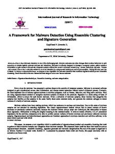
Figure 5: Distribution of cluster cohesion and separation (Feb09).

(a) Variant 1 (b) Variant 2 Figure 6: Example of malware variants that generate the very same network traffic, but also generate significantly different system events.

provide a comparison with the AV labels, and although our definition of cohesion and separation indexes attenuates the effect of AV label inconsistency (see Section 5), the results ultimately depend on the quality of the AV labels themselves. For example, we noticed that most pairs of clusters that have a low separation are due to the fact that their malware samples are labeled by the AV scanners as belonging to generic malware families, such as “Generic”, “Downloader”, or “Agent”. Overall, the distributions of the cohesion and separation indexes in Figure 5 show that most of the obtained behavioral malware clusters are very compact and fairly well separated, in terms of AV malware family labels. By combining this automated analysis with the manual analysis of those cases in which the separation index seemed to disagree with our clustering, we were able to confirm that our network-level clustering approach was indeed able to accurately cluster malware samples according to their network behavior.

requires more than 4 hours. Furthermore, although applying fine-grained clustering by itself requires less time than our three-step clustering approach (which includes meta-clustering) for three out of six datasets, our threestep clustering yields better signatures and a higher malware detection rate in all cases, as we discuss in Section 6.2. To analyze the quality of the final clusters generated by our system we make use of the cluster cohesion and separation defined in Section 5. Figure 5 shows a histogram of the cohesion index values (top graph) computed for each of the clusters obtained from the Feb09 malware dataset, and the distribution of the separation among clusters (bottom graph). Because of space limitations, we only discuss the cohesion and separation results from Feb09. The cohesion histogram only considers clusters that contain two or more malware samples (clusters containing only one sample have cohesion equal to 1 by definition). Ideally, we would like the value of cohesion for each cluster to be as close as possible to 1. Figure 5 confirms the effectiveness of our clustering approach. The vast majority of the behavioral clusters generated by our clustering system are very compact in terms of AV label graphs. This shows a strong agreement between our results and the malware family labels assigned to the malware samples by the AV scanners.

6.2

Network Signatures

In this section, we discuss how our network-level behavioral malware clustering can aid the automatic generation of network signatures. The main idea is to periodically extract signatures from newly collected malware samples, and to measure the effectiveness of such signatures for detecting the malicious HTTP traffic generated by current and future malware variants. Table 2 summarizes the results of the automatic signature generation process. For each month worth of HTTPbased malware, we considered only the malware clusters containing at least 2 samples. We do not consider signatures from singleton clusters because they are too specific and not representative of a family of malware. We ex-

Figure 5 also shows the distribution of the separation between pairs of malware clusters. Ideally we would like all the pairs of clusters to be perfectly separated (i.e., with a separation index equal to 1). Figure 5 (bottom graph) shows that most pairs of clusters are relatively well separated from each other. For example, 90% of all the cluster pairs from Feb09 have a separation index higher than 0.1. Both cluster cohesion and separation 9

dataset Feb09 Mar09 Apr09 May09 Jun09 Jul09

clusters (n > 1) 235 290 178 457 492 567

samples 3,494 2,074 1,285 2,725 2,438 3,430

signatures 544 721 378 1,013 974 1,367

pruned sig. 446 627 326 833 915 1,225

ated signatures as follows. Given the signatures in the set Sig Feb09, we matched them (using Snort) over the HTTP traffic traces generated by malware samples in Feb09, Mar09, Apr09, etc. We repeated the same process by testing the signatures extracted from a given month on the HTTP traffic generated by the malware collected in that month and in future months. We consider a malware sample to be detected if its HTTP traffic causes at least one alert to be raised. The detection results we obtained are summarized in Table 3. Take as an example the first row. The signature set Sig Feb09 “covers” (i.e., is able to detect) 85.9% of the malware samples collected in Feb09, 50.4% of the malware samples collected in Mar09, 47.8% of the malware samples collected in Apr09, and so on. Therefore, each of the signature sets we generated is able to generalize to new, never-beforseen malware samples. This is due to the fact that our network signatures aim to “summarize” the behavior of a malware family, instead of individual malware samples. As we discussed before, while malware variants from the same family can be generated at a high pace (e.g., using executable packing tools [16]), when executed they will behave similarly, and therefore can be detected by our behavioral network signatures. Naturally, as malware behavior evolves, the detection rate of our network signatures will decrease over time. Also, our approach is not able to detect “unique” malware samples, which behave differently from any of the malware groups our behavioral clustering algorithm was able to identify. Nonetheless, it is evident from Table 3 that if we periodically update our signatures with a signature set automatically extracted from the most recent malware samples, we can maintain a relatively high detection rate on current and future malware samples.

Table 2: Automatic signature generation and pruning results (processing times for signature extraction are included in Table 1, meta+sig column). Sig Sig Sig Sig Sig Sig

Feb09 Mar09 Apr09 May09 Jun09 Jul09

Feb09 85.9% -

Mar09 50.4% 64.2% -

Apr09 47.8% 38.1% 63.1% -

May09 27.0% 25.6% 26.4% 59.5% -

Jun09 21.7% 23.3% 27.6% 46.7% 58.9% -

Jul09 23.8% 28.6% 21.6% 42.5% 38.5% 65.1%

Table 3: Signature detection rate on current and future malware samples (1 month training)

tracted a signature set from each of the considered clusters as explained in Section 4. For example (Table 2, row 1), for the Feb09 malware dataset our clustering system found 235 clusters that contained at least 2 malware samples. The cumulative number of distinct samples contained in the 235 clusters was 3,494, from which the automatic signature generation process extracted a total of 544 signatures. After signature pruning (explained below) the number of signatures was reduced to 446. To perform signature pruning (see Section 4), we proceeded as follows. We collected a dataset of legitimate traffic by sniffing the HTTP requests crossing the webproxy of a large, well administered enterprise network with strict security policies for about 2 days, between November 25 and November 27, 2008. The collected dataset of legitimate traffic contained over 25.3 · 106 HTTP requests from 2,010 clients to thousands of different Web sites. We used existing automatic techniques for detecting malicious HTTP traffic and manual analysis to confirm that the collected HTTP traffic was actually as clean as possible. We split this dataset in two parts. We used the first day of traffic for signature pruning, and the second day to estimate the false positive rate of our pruned signatures (we will discuss our findings regarding false positives later in this section). To prune the 544 signatures extracted from Feb09, we translated the signatures in a format compatible with Snort [6], and then we used Sort’s detection engine to run our signatures over the first day of legitimate traffic. We then pruned those signatures that generated any alert, thus leaving us with 446 signatures. We repeated this pruning process for all the signature sets we extracted from the other malware datasets. In the following, we will refer to the pruned set of signatures extracted from Feb09 as Sig Feb09, and similarly for the other months Sig Mar09, Sig Apr09, etc.

False Positives To measure the false positives generated by our network signatures we proceeded as follows. For each of the signature sets Sig Feb09, Sig Mar09, etc., we used Snort to match them against the second day of legitimate HTTP traffic collected as described at the beginning of this Section. Table 4 summarizes the results we obtained. The first row reports the false positive rate, measured as the total number of alerts generated by a given signature set divided by the number of HTTP requests in the legitimate dataset. The numbers between parentheses represent the absolute number of alerts raised. On the other hand, the second row reports the fraction of distinct source IP addresses that were deemed to be compromised, due to the fact that some of their HTTP traffic matched any of our signatures. The numbers between parenthesis represent the absolute number of the source IPs for which an alert was raised. The results reported in Table 4 show that our signatures generate a low false positive rate. Furthermore, matching our signatures against one entire day of legit-

Detection Rate We measured the ability of our signatures to detect current and future malware samples. We measured the detection rate of our automatically gener10

FP rate Distinct IPs Processing Time

Sig Feb09 0% (0) 0% (0) 13 min

Sig Mar09 3 · 10−4 % (38) 0.3% (6) 10 min

Sig Apr09 8 · 10−6 % (1) 0.05% (1) 6 min

Sig May09 5 · 10−5 % (6) 0.2% (4) 9 min

Sig Jun09 2 · 10−4 % (26) 0.4% (9) 12 min

Sig Jul09 10−4 % (18) 0.3% (7) 38 min

Table 4: False positives measured on one day of legitimate traffic (approximately 12M HTTP queries from 2,010 different source IPs).

tures were generated) malware samples that AV scanners were not able to detect. We believe the poor performance of Sig Apr09 is due to the lower number of distinct malware samples that we were able to collect in Apr09. As a consequence, in that month we did not have a large enough number of training samples from which to learn good signatures.

imate traffic (about 12M HTTP queries from 2,010 distinct source IPs) can be done in minutes. This means that we would “keep up” with the traffic in real-time. Sig Sig Sig Sig

Feb09-Apr09 Mar09-May09 Apr09-Jun09 May09-Jul09

Apr09 70.8% -

May09 35.6% 61.6% -

Jun09 36.4% 48.6% 62.7% -

Jul09 35.1% 44.7% 48.6% 68.6%

Table 5: Signature detection rate on current and future malware samples (3 months training)

6.2.1 Real-World Deployment Experience We had the opportunity to test our network signatures in a large enterprise network consisting of several thousands nodes that run a commercial host-based AV system. We monitored this enterprise’s network traffic for a period of 4 days, from August 24 to August 28, 2009. We deployed our Sig Jun09 and Sig Jul09 HTTP signatures (using Snort) to monitor the traffic towards the enterprise’s web proxy. Overall, our signature set consisted of 2,140 Snort rules. We used the first 2 days of monitoring for signature-pruning (see Section 4), and the remaining 2 days to measure the number of false positives of the pruned signature set. During the pruning period, using a web interface to Snort’s logs, it was fairly easy to verify that 32 of our rules were actually causing false alerts. We then pruned (i.e., disabled) those rules and kept monitoring the logs for the next 2 days. In this 2-days testing period, overall the remaining signatures generated only 12 false alerts. During our 4 days monitoring, we also found that 4 of our network signatures detected actual malware behavior generated from 46 machines. In particular, we found that 25 machines were generating HTTP queries that matched a signature we extracted from two variants of TR/Dldr.Agent.boey [Avira]. By analyzing the payload of the HTTP requests we actually found that these infected machines seemed to be exfiltrating (POSTing) data to a notoriously spyware-related website. In addition, we found 19 machines that appeared to be infected by rogue AV software, one bot-infected machine that contacted its HTTP-based C&C server, and one machine that downloaded what appeared to be an update of PWS-Banker.gen.dh.dldr [McAfee].

Other Detection Results Table 5 shows that if we combine multiple signature sets, we can further increase the detection rate on new malware samples. For example, by combining the signatures extracted from the months of Apr09, May09, and Jun09 (this signature set is referred to as Sig Apr09-Jun09 in Table 5), we can increase the “coverage” of the Jun09 malware set from 58.9% (reported in Table 3) to 62.7%. Also, by testing the signature set Sig Apr09-Jun09 against the malware traffic from Jul09 we obtained a detection rate of 48.6%, which is significantly higher than the 38.5% detection rate obtained using only the Sig Jun09 signature set (see Table 3). In addition, matching our largest set of signatures Sig May09-Jul09, consisting of 2,973 distinct Snort rules, against one entire day of legitimate traffic (about 12 million HTTP queries) took less than one hour. This shows that our behavioral clustering and subsequent signature generation approach, though not a silver bullet, is a promising complement to other malware detection techniques, such as AV scanners, and can play an important role in a defense-in-depth strategy. This is also reflected in the results reported in Table 6, which represent the detection rate of our network signatures with respect to malware samples that were not detected by any of the three AV scanners available to us. For example, using the signature set Sig Feb09 , we are able to detect 54.8% of the malware collected in Feb09 that were not detected by the AV scanners, 52.8% of the undetected (by AVs) samples collected in Mar09, 29.4% of the undetected samples collected in Apr09, etc. Sig Sig Sig Sig Sig Sig

Feb09 Mar09 Apr09 May09 Jun09 Jul09

Feb09 54.8% -

Mar09 52.8% 54.1% -

Apr09 29.4% 20.6% 41.9% -

May09 6.1% 5.0% 5.8% 66.7% -

Jun09 3.6% 3.1% 3.8% 38.8% 48.9% -

Jul09 4.0% 5.4% 5.2% 16.1% 21.8% 62.9%

6.2.2 Comparison with other approaches. Table 7, third row, shows the next month detection rate (NMDR) for signatures generated by applying finegrained clustering alone to each of our malware datasets. For example, given the malware dataset Feb09, we directly applied fine-grained clustering to the related malicious traffic traces, instead of applying our three-step clustering process. Then, we extracted a set of signatures from each fine-grained cluster, and we tested the ob-

Table 6: Detection rate on malware undetected by all AVs.

We can see from Table 6 that, apart from the signatures Sig Apr09, all the other signature sets allow us to detect between roughly 20% and 53% of future (i.e., collected in the next month, compared to when the signa11

tained signature set on the HTTP traces generated by executing the malware samples from the Mar09 dataset. We repeated this process for all the other malware datasets (notice that the NMDR for Jul09 is not defined in table Table 7, since we did not collect malware from August 2009). By comparing the results in Table 7 with Table 3, we can see that the signatures obtained by applying our three-step clustering process always yield a higher detection rate, compared to signatures generated by applying the fine-grained clustering algorithm alone. Clusters Time NMDR

Feb09 2,934 4h4min 38.4%

Mar09 2,352 1h52min 25.7%

Apr09 1,485 1h1min 24.2%

May09 2,805 3h9min 46.2%

Jun09 2,719 3h18min 36.3%

Jul09 3,343 2h57min -

Table 7: Results obtained using only fine-grained clustering, instead of the three-step clustering process (NMDR = next month detection rate).

We also compared our approach to [10]. We randomly selected around four thousand samples from the Feb09 and May09 malware datasets. Precisely, we selected 2,038 samples from Feb09 and 1,978 samples from May09. We then shared these samples with the authors of [10], who kindly agreed to provide the clustering results produced by their system. The results they were able to share with us were in the form of a similarity matrix for each of the malware datasets we sent them. We then applied single linkage hierarchical clustering to each of these similarity matrices to obtain the related dendrogram. In order to find where to cut the obtained dendrogram, we used two different strategies. First, we applied the DB index [17] to automatically find the best dendrogram cut. However, the results we obtained were not satisfactory in this case, because the clusters were too “tight”. Only very few clusters contained more than one sample, thus yielding very specific signatures with a low detection rate. We then decided to select the threshold manually using our domain knowledge. This manual tuning process turned out to be very time-consuming, and therefore we finally decided to simply use the similarity threshold value t = 0.7, which was also used in [10]. A manual analysis confirmed that with this threshold we obtained much better results, compared to using the DB index. We then extracted network signatures from the malware clusters obtained using both our three-step networklevel clustering system, our fine-grained clustering only, and [10] (in all cases, we used the HTTP traffic traces collected using our malware analysis system to extract and test the network signatures). All clustering approaches were applied to the same reduced datasets described earlier. The results of our experiments are reported in Table 8. In the first row, “Sig Feb09 netclusters” indicates the dataset of signatures extracted from the (reduced) Feb09 dataset using our three-step network-level clustering. “Sig Feb09 net-fg-clusters”

represents the set of signatures extracted using our finegrained clustering only, while “Sig Feb09 sys-clusters” indicates the signatures extracted from malware clusters obtained using a system-level clustering approach similar to [10]. We then tested the obtained signature sets on the traffic traces of the entire malware datasets collected in Feb09 and Mar09. We repeated a similar process to obtain and test the “Sig May09 netclusters”, “Sig May09 net-fg-clusters”, and “Sig May09 sys-clusters” using malware from the May09 dataset. From Table 8 we can see that the signatures obtained using our three-step clustering process yield a higher detection rate in all cases, compared to using only fine-grained clustering, and to signatures obtained using a clustering approach similar to [10]. Sig Sig Sig Sig Sig Sig

Feb09 net-clusters Feb09 net-fg-clusters Feb09 sys-clusters May09 net-clusters May09 net-fg-clusters May09 sys-clusters

Feb09 78.6% 60.1% 56.9% -

Mar09 48.9% 35.1% 33.9% -

May09 56.0% 50.8% 32.7%

Jun09 44.3% 42.5% 32.0%

Table 8: Malware detection rate for network signatures generated using our three-step network-level clustering (net-clusters), only fine-grained network-level clustering (net-fg-clusters), and clusters generated using [10] (sys-clusters).

It is worth noting that while it may be possible to tune the similarity threshold t to improve the systemlevel clusters, our network-level system can automatically find the optimum dendrogram cut and yield accurate network-level malware signatures. We also applied Polygraph [24] to a subset of (only) 49 malware samples from the Virut family. Polygraph ran for more than 2 entire weeks without completing. It is clear that Polygraph’s greedy clustering algorithm is not suitable for the problem at hand, and that without the preprocessing provided by our clustering system generating network signatures to detect malware-related outbound HTTP traffic would be much more expensive. 6.2.3 Qualitative Analysis In this section, we analyze some of the reasons why system-level clustering may perform worse than network-level clustering, as shown in Table 8. In some cases, malware variants that generate the same malicious network traffic may generate significantly different system-level events. Consider the example in Figure 6, which reports information about the system and network events generated by two malware variants v1 , and v2 (which are part of our Feb09 dataset). v1 is labeled as Generic FakeAlert.h by McAfee and as TR/Dropper.Gen by Avira (Trend did not detect it), whereas v2 is labeled as DR/PCK.Tdss.A.21 by Avira (neither McAfee nor Trend detected this sample). When executed, the first sample runs in the background and does not display any message to the user. On the 12

may be triggered by events [11] such as a particular date, the way the user interacts with the infected machine, etc. In such cases, techniques similar to the ones proposed in [11] may be used to identify and activate such triggers. Trigger-based malware analysis is outside the scope of this paper, and is therefore left to future work. Because we perform an analysis of the content of HTTP requests and responses, encryption represents our main limitation. Some malware writers may decide to use the HTTPS protocol, instead of HTTP. However, it is worth noting that using HTTPS may play against the malware itself, since many networks (in particular enterprise networks) may decide to allow only HTTPS traffic to/from certified servers. While some legitimate websites operate using self-signed public keys (e.g., to avoid CA signing costs), these cases can be handled by progressively building a whitelist of authorized self-signed public keys. However, we acknowledge this approach may be hard to implement in networks (e.g., ISP networks) where strict security policies may not be enforced. Our signature pruning process (see Section 4) relies on testing malware signatures against a large dataset of legitimate traffic. However, collecting a completely clean traffic dataset may be difficult in practice. In turn, performing signature pruning using a non-clean traffic dataset may cause some malware signatures to be erroneously filtered out, thus decreasing our detection rate. There are a number of practical steps we can follow to mitigate this problem. First, since we are mostly interested in detecting new malware behavior, we can apply our signature pruning process over a dataset of traffic collected a few months before. The assumption is that this “old” traffic will not contain traces of future malware behavior, and therefore the related malware signatures extracted by our system will not be filtered out. On the other hand, we expect the majority of legitimate HTTP traffic to be fairly “stable”, since the most popular Web sites and applications do not change very rapidly. Another approach we can use is to collect traffic from many different networks, and only filter out those signatures that generate false positives in the majority of these networks. The assumption here is that the same new malware behavior may not be present in the majority of the selected networks at the same time. Evasion attacks, such as noise-injection attacks [28] and other similar attacks [25], may affect the results of our clustering system and network signatures. Because we run the malware in a protected environment, it may be possible to identify what HTTP requests are actually performed to send or receive information critical for the correct functioning of the malware using dynamic taint analysis [13]. This may allow us to correlate network traffic with system activities performed by the malware, and to identify whether the malware is injecting ran-

other hand, the second sample is a Trojan that presents the user with a window pretending to be the installation software for an application called Aquaplay. However, regardless of whether the user chooses to complete the installation or not, the malware starts running and generating HTTP traffic. The set of operations each variant performs on the system are significantly different (because of space limitations, Figure 6 only shows filesystem events), and therefore these two samples would tend to be separated by system-level behavioral clustering. However, the HTTP traffic they generate is exactly the same. Both v1 and v2 send the same amount of data to an IP address apparently located in Latvia, using the same two POST requests. It is clear that these two malware samples are related to each other, and our network-level clustering system correctly groups them together. We speculate that this is due to the fact that some malware authors try to spread their malicious code by infecting multiple different legitimate applications (e.g., different games) with the same bot code, for example, and then publishing the obtained trojans on the Internet (e.g., via peer-to-peer networks). When executed, each trojan may behave quite differently from a system point of view, since the original legitimate portions of their code are different. However, the malicious portions of their code will contact the same C&C. Another factor to take into account is that malware developers often reuse code written by others and customize it to fit their needs. For example, they may reuse the malicious code used to compromise a system (e.g., the rootkit installation code) and replace some of the malicious code modules that provide network connectivity to a C&C server (e.g., to replace an IRC-based C&C communication with code that allows the malware to contact the C&C using the HTTP protocol). In this case, while the system-level activities of different malware may be very similar (because of a common system infection code base), their network traffic may look very different. In this case, grouping these malware in the same cluster may yield overly generic network signatures, which are prone to false positives and will likely be filtered out by the signature pruning process. Although it is difficult to measure how widespread such malware propagation strategies are, it is evident that system-level clustering may not always yield the desired results when the final objective is to extract network signatures.

7

Limitations and Future Work

Similarly to previous work that relies on executing malware samples to perform behavioral analysis [9, 10, 20], our analysis is limited to malware samples that perform some “interesting actions” (i.e., malicious activities) during the execution time T . Unfortunately, these interesting actions (both at the system and network level) 13

domly generated/selected elements into the network traffic. However, taint analysis may be evaded [12] and misled using sophisticated noise-injection attacks. Systemlevel malware clustering (such as [9, 10]) and signature generation algorithms may also be affected by such attacks, e.g., by creating “noisy” system events that do not serve real malicious purposes, but simply try to mislead the clustering process and the generation of a good detection model. Noise injection attacks are a challenging research problem to be addressed in future work.

8

[6] Snort IDS. http://www.snort.org. [7] Trend Micro Anti-Virus. http://www.trendmicro.com. [8] Zeus Tracker. https://zeustracker.abuse.ch/faq. php. [9] M. Bailey, J. Oberheide, J. Andersen, Z. M. Mao, F. Jahanian, and J. Nazario. Automated classification and analysis of internet malware. In Recent Advances in Intrusion Detection, 2007. [10] U. Bayer, P. Milani Comparetti, C. Hlauschek, C. Kruegel, and E. Kirda. Scalable, behavior-based malware clustering. In Network and Distributed System Security Symposium, 2009. [11] D. Brumley, C. Hartwig, Z. Liang, J. Newsome, D. Song, and H. Yin. Automatically identifying trigger-based behavior in malware. Botnet Detection, 2008. [12] L. Cavallaro, P. Saxena, and R. Sekar. On the limits of information flow techniques for malware analysis and containment. In International conference on Detection of Intrusions and Malware, and Vulnerability Assessment, 2008. [13] J. Clause, W. Li, and A. Orso. Dytan: a generic dynamic taint analysis framework. In International symposium on Software testing and analysis, 2007. [14] D. Danchev. Web based botnet command and control kit 2.0, August 2008. http://ddanchev.blogspot.com/2008/ 08/web-based-botnet-command-and-control. html. [15] G. Gu, R. Perdisci, J. Zhang, and W. Lee. Botminer: clustering analysis of network traffic for protocol- and structureindependent botnet detection. In USENIX Security, 2008. [16] F. Guo, P. Ferrie, and T. Chiueh. A study of the packer problem and its solutions. In Recent Advances in Intrusion Detection, 2008. [17] M. Halkidi, Y. Batistakis, and M. Vazirgiannis. On clustering validation techniques. J. Intell. Inf. Syst., 17(2-3):107–145, 2001. [18] A. K. Jain and R. C. Dubes. Algorithms for clustering data. Prentice-Hall, Inc., 1988. [19] A. K. Jain, M. N. Murty, and P. J. Flynn. Data clustering: a review. ACM Comput. Surv., 31(3):264–323, 1999. [20] J. P. John, A. Moshchuk, S. D. Gribble, and A. Krishnamurthy. Studying spamming botnets using botlab. In USENIX Symposium on Networked Systems Design and Implementation (NSDI), 2009. [21] E. Kirda, C. Kruegel, G. Banks, G. Vigna, and R. A. Kemmerer. Behavior-based spyware detection. In USENIX Security, 2006. [22] V. Laurikari. TRE. http://www.laurikari.net/tre/. [23] Z. Liand, M. Sanghi, Y. Chen, M. Kao, and B. Chavez. Hamsa: Fast signature generation for zero-day polymorphicworms with provable attack resilience. In IEEE Symposium on Security and Privacy, 2006. [24] J. Newsome, B. Karp, and D. Song. Polygraph: Automatically generating signatures for polymorphic worms. In IEEE Symposium on Security and Privacy, 2005. [25] J. Newsome, B. Karp, and D. Song. Paragraph: Thwarting signature learning by training maliciously. In Recent Advances in Intrusion Detection (RAID), 2006. [26] J. Oberheide, E. Cooke, and F. Jahanian. CloudAV: N-Version antivirus in the network cloud. In USENIX Security, 2008. [27] D. Pelleg and A. W. Moore. X-means: Extending k-means with efficient estimation of the number of clusters. In International Conference on Machine Learning, 2000. [28] R. Perdisci, D. Dagon, W. Lee, P. Fogla, and M. Sharif. Misleadingworm signature generators using deliberate noise injection. In IEEE Symposium on Security and Privacy, 2006. [29] S. Singh, C. Estan, G. Varghese, and S. Savage. Automated worm fingerprinting. In ACM/USENIX Symposium on Operating System Design and Implementation, December 2004. [30] Symantec. Symantec Global Internet Security Threat Report trends for 2008, April 2009. [31] S. Wu and U. Manber. Agrep – a fast approximate patternmatching tool. In USENIX Technical Conference, 1992. [32] Y. Xie, F. Yu, K. Achan, R. Panigrahy, G. Hulten, and I. Osipkov. Spamming botnets: signatures and characteristics. In ACM SIGCOMM conference on data communication, 2008. [33] V. Yegneswaran, J. T. Giffin, P. Barford, and S. Jha. An architecture for generating semantics-aware signatures. In USENIX Security Symposium, 2005. [34] H. Yin, D. Song, M. Egele, C. Kruegel, and E. Kirda. Panorama: capturing system-wide information flow for malware detection and analysis. In ACM Conference on Computer and Communications Security, 2007.

Conclusion

In this paper, we presented a network-level behavioral malware clustering system that focuses on HTTP-based malware and clusters malware samples based on a notion of structural similarity between the malicious HTTP traffic they generate. Through network-level analysis, our behavioral clustering system is able to unveil similarities among malware samples that may not be captured by current system-level behavioral clustering systems. Also, we proposed a new method for the analysis of malware clustering results. The output of our clustering system can be readily used as input for algorithms that automatically generate network signatures. Our experimental results on over 25,000 malware samples confirm the effectiveness of the proposed clustering system, and show that it can aid the process of automatically extracting network signatures for detecting HTTP traffic generated by malware-compromised machines.

Acknowledgements We thank Paolo Milani Comparetti for providing the results that allowed us to compare our system to [10], Philip Levis for his help with the preparation of the final version of this paper, and Junjie Zhang and the anonymous reviewers for their constructive comments. This material is based upon work supported in part by the National Science Foundation under grants no. 0716570 and 0831300, the Department of Homeland Security under contract no. FA8750-08-2-0141, the Office of Naval Research under grant no. N000140911042. Any opinions, findings, and conclusions or recommendations expressed in this material are those of the authors and do not necessarily reflect the views of the National Science Foundation, the Department of Homeland Security, or the Office of Naval Research.

References [1] Avira Anti-Virus. http://www.avira.com. [2] Collaborative Malware Collection and Sensing. https:// alliance.mwcollect.org. [3] Koobface. http://blog.threatexpert.com/2008/ 12/koobface-leaves-victims-black-spot.html. [4] McAfee Anti-Virus. http://www.mcafee.com. [5] Project Malfease. http://malfease.oarci.net.

14