Bayesian Variable Order Markov Models
Christos Dimitrakakis University of Amsterdam
Abstract We present a simple, effective generalisation of variable order Markov models to full online Bayesian estimation. The mechanism used is close to that employed in context tree weighting. The main contribution is the addition of a prior, conditioned on context, on the Markov order. The resulting construction uses a simple recursion and can be updated efficiently. This allows the model to make predictions using more complex contexts, as more data is acquired, if necessary. In addition, our model can be alternatively seen as a mixture of tree experts. Experimental results show that the predictive model exhibits consistently good performance in a variety of domains. We consider Bayesian estimation of variable order Markov models (see Begleiter et al., 2004, for an overview). Such models create a tree of partitions, where the disjoint sets of every partition correspond to different contexts. We can associate a sub-model or expert with each context in order to make predictions. The main contribution of this paper is a conditional prior on the Markov order—or equivalently the context depth. This is based on a recursive construction that estimates, for each context at a certain depth k, whether it makes better predictions than the predictions of contexts at depths smaller than k. This simple model defines a mixture of variable order Marko models and its parameters can be updated in closed form in time O (D) for trees of depth D with each new observation. For unbounded length � contexts, the complexity of the algorithm is O T 2 for an input sequence of length T . Furthermore, it exhibits robust performance in a variety of tasks. Finally, the model is easily extensible to controlled processes. Appearing in Proceedings of the 13th International Conference on Artificial Intelligence and Statistics (AISTATS) 2010, Chia Laguna Resort, Sardinia, Italy. Volume 9 of JMLR: W&CP 9. Copyright 2010 by the authors.
The following section presents our setup for the sequence prediction problem and introduces notation. Section 2 defines the proposed Bayesian variable order Markov model (henceforth BVMM) and derives a closed form sequential update for the model parameters. Section 3 gives a brief overview of other tree based models, as well as a standard Markov chain mixture, and discusses their relation to BVMMs. Experimental comparisons between various models are given in Section 4, on a number of sequential prediction problems. The paper concludes with Section 5, which also discusses extensions and applications to reinforcement learning.
1
INTRODUCTION
We consider sequences of observations x1 , x2 , . . ., with xt ∈ X . We assume the existence of a suitable σalgebra BX such that (X , BX ) is measurable. In particular, most of the following development assumes a finite X . Subsequences are denoted by xk:t for k ≤ t and the concatenations of sequences are denoted by · ◦ ·. For example xk:t+1 = xk:t ◦ xt+1 . In addition, let S∞ X 0 , ∅, X n , ×n X , Xk∗ , n=k X n and X ∗ , X0∗ . We use bold symbols for arbitrary-length sequences x and we denote the length of any x ∈ X ∗ by ℓ (x). Suffixes. We call x a suffix of x′ , and write x ≺ x′ iff ℓ (x) ≤ ℓ (x′ ) and xℓ(x)+1−i = x′ℓ(x′ )+1−i for all i ∈ {1, . . . , ℓ (x)}. Finally, we write x ∩ x′ to denote the largest common suffix of x, x′ ∈ X ∗ . If x and x′ have no common suffix then x∩x′ = 0 and 0◦x = x◦0 = x for any x ∈ X ∗ . Definition 1. A suffix set S on X is a set of sequences c ∈ X ∗ . S is proper iff c ∩ c′ = 0 for all c, c′ ∈ S. We call S complete iff, ∀x ∈ X ∗ , ∃c ∈ S such that c ≺ x. We consider a complete, but not proper, suffix set S, which may be infinite, constructed via a tree T = (V, E), of depth D, E. The � with nodes V and edges set of nodes V = vi : i = 0, 1, . . . , |X |D is such that the node vi ∈ V corresponds to a unique sequence ci ∈ X ∗ . Specifically, the root node v0 corresponds to c0 = 0, the empty sequence. All inner nodes have |X |
Bayesian Variable Order Markov Models
children, such that if vj is the k-th child of node vi , then cj = k ◦ vi . Thus, there are t + 1 suffixes in S for each sequence x1:t ∈ X t and the tree can be viewed ∗ as a tree of partitions of XD . Indeed, the suffixes par∗ tition XD into sets Xi , {c ∈ X ∗ : ci ≺ c}, such that Pk , {Xi : ℓ (ci ) = k, ci ∈ S} is the partition induced by the set of nodes at depth k of the tree. Context models. The general idea of such models is to associate an expert µi with a context ci , such that, for a given observation history, only certain experts will have matching contexts. For the problem of sequence prediction, the context ci is the suffix at the node vi of the tree and the expert µi defines a probability measure P(· | µi ) on (X , BX ) that predicts the next observations. Given any sequence x1:t , only a subset of experts M(x1:t ) , (µi : ci ≺ x1:t ) will have contexts that are suffixes of x1:t . For any active expert µk ∈ M(x1:t ), we shall use: ptk (x) , P(xt+1 = x | µk , x1:t )
(1)
to denote the (marginal) posterior probability of possible next observations xt+1 , according to expert µk , given the history of previous t observations. Example 1. When X = {1, . . . , K}, we can use a Dirichlet distribution Dir (αkt ) over multinomial paramt eters for each µk , where αkt , (αk,j )K j=1 is the vector of Dirichlet parameters for expert k at time t. The corresponding marginal probability distribution is: ptk (xt+1
t αk,x
= x) = PK
j=1
t αk,j
,
(2)
for all k ∈ {1, . . . , K}. Given a sequence x1:T , the parameters of the expert at each context are T 0 αi,k = αi,k +
T X
I {ci ≺ x1:t ∧ xt+1 = k} ,
(3)
2
BAYESIAN VARIABLE ORDER MARKOV MODELS
We first define variable order Markov models as a set of experts on a suffix tree. Subsequently, we define a mixture of such models, associated with a set of weights and we give a procedure for updating the weights given new observations. Definition 2. A Variable order Markov Model (VMM) over X ∗ is composed of: 1. A complete suffix set S = {ci : i = 1, . . . , N }. 2. A set of experts M = {µi : i = 1, . . . , N }, indexing a set of probability distributions: {P(xt+1 | µi ) : µi ∈ M}. For the discrete case in particular, each expert µi ∈ M defines a multinomial distribution with parameters τi ∈ [0, 1]|X | s.t. kτi k1 = 1 and P(xt+1 = j | µi ) = τi,j . There is a one-to-one correspondence between each context ci and each expert µi . For any history x1:t ∈ X t , the we use the surjection I : X ∗ → {1, . . . , N } to denote the index I(t) , max {i : ci ≺ x1:t } of the only active expert (i.e. the active expert is the one with the largest matching suffix). The distribution of next observations is: P(xt+1 | x1:t ) , P(xt+1 | µI(t) )
(5)
To obtain a distribution of VMMs that can be updated in closed form, we define the following structure. Definition 3 (BVMM). A Bayesian variable order Markov model over X ∗ is composed of: 1. A suffix tree T = (V, E), of depth D with a set of nodes V = {vi : i = 0, 1, . . . , N }, with N = X D , and a set of edges E.
t=1
n o 0 where αi,k is a set of prior parameters, typically set to values in [0, 1].
For any conditional probability distribution P(µ|x1:t ) over the set of active experts M(x1:t ), we obtain the marginal probability of the next observations: X P(xt+1 |x1:t ) = ptk (xt+1 ) P(µk |x1:t ). (4) µk ∈M(x1:t )
This natural idea is used in the context tree weighting algorithm (Willems et al., 1995), which employs Dirichlet models for µ. It however only considers a fixed P(µ|x1:t ). We shall introduce a simple construction that allows us to update both P(µ|x1:t ) and the experts µ efficiently.
2. A complete suffix set S = {ci : i = 0, 1, . . . , N }. 3. A set of models M = {µi : i = 0, 1, . . . , N }. For |X | discrete X , these are Dir (αi ) with αi ∈ R+ . 4. A set of weights {wi ∈ [0, 1] : i = 0, 1, . . . , N }.
W
=
There is a one-to-one correspondence between each node vi , a suffix ci , an expert µi and a weight wi . For any observations x1:t ∈ X t , the set of active experts is M(x1:t ) , (µI(0,t) , . . . , µI(t,t) ), where I : X ∗ × N → {0, . . . , N } is a surjection such that cI(0,t) = 0 and cI(k+1,t) = xt−k ◦ cI(k,t) . In order to generate a new observation xt+1 , given x1:t , we define the auxiliary indicator variable st =
Christos Dimitrakakis
(st,0 . . . , st,t ), such that: xt+1 ∼ P(xt+1 | x1:t , µI(k,t) ) if st,k = 1. The following properties hold for s: P(st,t = 1 | x1:t ) = wI(t,t) , P(st,k = 1 | st,k+1 = 0, x1:t ) = wI(k,t) , P(st,k = 1 | ∃j > k : sj = 1) = 0, w0 = 1. The probability of the data being generated by the k-th model, according to the ordering implied by x1:t , is: t Y
P(st,k = 1 | x1:t ) = wI(k,t)
(1 − wI(j,t) ),
(6)
j=k+1
where
Qt
j=t+1 (1−wI(j,t) )
= 1 for notational simplicity.
Intuitively, s can be seen as a stopping variable. Given an observation x1:t , we form the chain of active experts M(x1:t ). Starting from the last model, µI(min(t,D),t) , and for every model µI(k,t) ∈ M(x1:t ), we stop with probability wI(k,t) and generate xt+1 ∼ pI(k,t) (xt+1 ). Otherwise, we move to µI(k−1,t) . If k = 0, the next observation is generated from the root model µ0 . P Remark 1. By construction, k P(st,k � = 1) = 1, for any set of weights wI(k,T ) ≥ 0 : k > 0 . Proof. The proof proceeds by induction. Without loss of generality, we only consider tP ≤ D, since we can set t wt = 0 for t > D. When t = 0, k=0 P(st,k ) = w0 = 1 by definition, where we used P(st,k ) ≡ P(st,k = 1) for compactness. For other t: t+1 X
k=0
P(st,k |x1:t ) =
t+1 X
k=0
wI(k,t)
t+1 Y
t wI(k,t) = P(µI(k,t) | x1:t , Bk ).
= (1 − wI(t+1,T ) )
P(st,k ) + wI(t+1,T ) ,
k=0
Pt
k=0
P(xt+1 =x|x1:t ) =
Proof. W and S define a distribution over complete context sets of maximum suffix length D. To see this, ˆ Since w0 = let us construct a random context set S. ˆ 1, S is always complete and the probability of each context being in Sˆ can be derived via (6) as: Y ˆ ∝ wi P(ci ∈ S) (1 − wj ). (7)
t ptI(k,t) (x)wI(k,t)
t Y
t (1 − wI(n,t) ).
n=k+1
The following theorem gives a procedure for updating W in closed form. Theorem 1. The weight parameters W of any BVMM can be recursively updated in closed form according to: t+1 wI(k,t) , P(µI(k,t) |x1:t+1 , Bk )
(9)
t ptI(k,t) (xt+1 )wI(k,t) t t pI(k,t) (xt+1 )wI(k,t) + P(xt+1 |x1:t , Bk−1 )(1
t − wI(k,t) )
Proof. First of all, note that Bt is trivially true at time t. For Bk with k < t, it is easy to see that the following recursions hold: t P(Bk−1 |x1:t ) = P(Bk |x1:t )(1 − wI(k,t) )
P(xt+1 |x1:t , Bk ) =
(10a)
t ptI(k,t) (xt+1 )wI(k,t)
+ P(xt+1 |x1:t , Bk−1 )(1 −
(10b) t wI(k,t) ),
where we used (8) and that P(xt+1 |µI(k,t) , x1:t , Bk ) = P(xt+1 |µI(k,t) , x1:t ) = ptI(k,t) (xt+1 ), as given the k-th expert, the next observations do not depend on previous experts. Using (10) and Bayes’ theorem, we have: t+1 wI(k,t) , P(µI(k,t) |x1:t+1 , Bk )
=
j:ci ≺cj
ˆ generate multinomial paramFinally, for all ci ∈ S, eters τi ∼ Dir (αi ). These two sets are sufficient for specifying a VMM.
t X
k=0
P(st,k ) = 1.
Remark 2. A BVMM of depth D defines a distribution over VMMs.
(8)
Using (6), we can write the marginal predictive distribution (4) of our model at time t, in terms of the weights:
(1 − wI(n,T ) ) t X
Update procedure
We now consider a recursive procedure for updating the parameters of a BVMM. For this reason, we use a superscript t to refer to the value of parameters at time t. Furthermore, we need a way to refer to the observations being generated an expert in a particular subset. This leads us to the following construction, which is central in the remaining development: Let Bk , I {∃i ≤ k : st,k = 1} denote the event that the data is generated by one of�the experts with context size at most k, i.e. that µ ∈ µI(0,t) , . . . , µI(k,t) . This allows us to interpret the weights as the posterior of the k-th model (where k indexes the active context experts M(x1:t )), given the observation history x1:t and the fact that the model order is not larger than k:
=
n=k+1
which obviously equals 1 if
2.1
=
P(xt+1 |µI(k,t) , x1:t , Bk ) P(µI(k,t) |x1:t , Bk ) P(xt+1 |x1:t , Bk ) t ptI(k,t) (xt+1 )wI(k,t) t t ptI(k,t) (xt+1 )wI(k,t) + P(xt+1 |x1:t , Bk−1 )(1 − wI(k,t) )
Bayesian Variable Order Markov Models
Updating ptk (x) is easy if µk is Dirichlet with parameters αk , {αk,i : i = 1, . . . , |X |}, as described in Example 1. Finally, note that due to Remark 1, the weights always define a proper posterior probability distribution over the experts and additionally, a distribution over VMMs due to Remark 2. Remark 3. At each step t, the update complexity is O (min{D, t}), so the complexity for a sequence of � length T is O min{T 2 , T D} .
3
RELATED MODELS
This section gives a brief overview of models related to BVMMs. Of these, the closest models are the following: (a) The Bayesian Markov chain mixture, which uses a standard prior over Markov order. (b) Dirichlet process models, which employ sampling. (c) The context tree weighting algorithm (Willems et al., 1995), which has fixed weights. We shall now discuss the related models in more detail. Bayesian Markov chain mixture. A simpler type of Bayesian model for sequence prediction is a mixture over Markov chains (henceforth BMCM). Let a set of experts {µk : k = 0, . . . , D}, and a multinomial prior distribution with parameters φ0 = (φ0k )D k=0 . Each expert µk is a distribution over the parameters of Markov chains of order k for a discrete observation set X . In particular, we consider a productof-Dirichlets conjugate prior, with parameters αkt , o n
BVMMs with respect to the adaptation of the experts µ, when those are Dirichlet-multinomial. While CTW uses a closed-form update, the weights used in CTW are fixed. The prediction by partial matching (PPM) algorithm (Cleary and Witten, 1984), includes a closed-form weight update, which is however ad-hoc (Begleiter et al., 2004, p.392). Other variants are examined in (Begleiter et al., 2004) which in addition supplies an experimental comparison between methods. A final related model is Variable length Markov chains (B¨ uhlmann and Wyner, 1999) (henceforth VMC), which however utilises growing and subsequent pruning of the context tree. It is thus a batch (offline) algorithm. Tree experts. A tree expert is a collection of a finite number of experts, with each expert being a predictive tree, whose nodes are of two types: leaf nodes (which have no children) and inner nodes (which all have n children). Decisions at inner nodes concern only which child to proceed to, while the decisions at leaf nodes concern a prediction of the next observation. A VMM can be seen as a particular type of tree expert and a BVMM as a mixture of tree experts. A low regret prediction algorithm for such models is given in (CesaBianchi and Lugosi, 2006, ch. 5.3).
This model is simpler than a BVMM. In fact, it can be seen as a BVMM with the weights of all contexts at a certain depth k being equal. Thus, a potential problem is that a large amount of data is required for the µk+1 to start making globally better predictions than µk . Intuitively, we could do better by switching to larger order models for some contexts only. This can be achieved if we allow our belief over model order to depend on the history, something taken care of automatically in BVMMs.
Dirichlet process models. An important class of priors over distriutions are Polya trees (Ferguson, 1974). Just as in BVMMs, a distribution is defined over a partition tree. However, there is only one set of parameters for each node, which relates to the child node which will be next visited. This allows closed form updates, but lacks the additional expressiveness possible with BVMMs. Dirichlet processes are also used in the infinite hidden Markov model (IHMM, Beal et al., 2001) and the infinite Markov model (IMM, Mochihashi and Sumita, 2008). In particular, the IMM uses a similar structure, with the difference that a Beta prior on the stopping variable s is used. Inference in both of these models requires sampling instead. Thus, as long as one is only interested in prediction, rather than state estimation, BVMMs amount to a significant improvement over I(H)MMs in terms of computation. However, another approach close to the BVMM is the stochastic memoizer (SM), proposed by Wood et al. (2009), which, although it also employs sampling, it is much more efficient in terms of computation.
Other variable length Markov chains models. One closely related model is the context tree weighting (henceforth CTW) algorithm (Willems et al., 1995). CTW employs smooth maximum likelihood estimation at each context and so is equivalent to
Other models. In a different setting, learning mixtures of trees has been explored using EM in (Meila and Jordan, 2001), with a similar construction to the BVMM and the IMM, while (Friedman and Koller, 2003) extended the work to the more general problem
T 0 t = αk,z + αk,z : z ∈ X k , updated according to αk,z PT t=1 I {z ≺ x1:t ∧ xt+1 = k} and with (marginal) pre-
dictive distribution ptk (xt+1 = i|z ≺ x1:t ) = The mixture is updated via Bayes’ rule: pt (xt+1 )φtk φt+1 , PD k k t t j=0 pj (xt+1 )φj
αt P i,zt . j αj,z
(11)
Christos Dimitrakakis
of learning network structure, for which they employed Markov chain Monte Carlo approaches. Finally, there are some parallels with the autoregressive literature, where the prediction problem is the same, but X ⊂ Rn , such as the work of Mena and Walker (2005), which utilised a Dirichlet process mixture latent variable.
4
EXPERIMENTS
We evaluated the method on a number of sequence prediction domains.1 The objective was to compare its performance against commonly used approaches in the target domain. Our evaluation criterion was the total error made by each algorithm in online prediction. For comparative purposes, we employed two domains. The first was stochastically generated hidden Markov models, for which there exist approximate inference methods in the target model class. The second domain was fixed sequences of text and gene data. 4.1
HIDDEN MARKOV MODEL
In this domain, data is generated from a hidden Markov model (hence forth HMM) ν ∗ , with a discrete set of states s ∈ S and observations x ∈ X . Experiments were performed for |S| ∈ {2, 4, 8} and |X | ∈ {2, 4, 8}. There were 100 runs performed for each choice of X , S. For each run, a HMM was stochastically generated in order to ensure that: (a) There would be some stationarity in every state, so as to make sequences more predictable. (b) States would be sufficiently differentiable from each other. For the n-th run of each experiment, a HMM νn∗ with transition and observation matrices P and Q, such that Pij , νn∗ (st+1 = j|st = i) and Qij , νn∗ (xt = j|st = i), was used to generate the observation sequence x1:t by setting s0 = 1 and sampling st+1 ∼ νn∗ (st+1 |st ), and xt ∼ νn∗ (xt |st ). In order to ensure that the HMMs had the desired structure, the matrices were generated as follows. First, a stationarity parameter β was generated uniformly in the interval P [ 21 , 1). The entries of P were set to Pij = pˆij / k pˆik , with pˆi,j = I {i = j} β+exp(zi,j ), with zi,jP ∼ Uni (0, 1). The entries of Q were set to Qij = qˆij / k qˆik , with qˆi,j = I {i = j} + ζi,j , with ζi,j ∼ Uni (0, 1/10). For each run, we calculated the cumulative loss ℓ of each model ν assigning probabilities ν t (xt+1 ) to outcomes given the history x1:t , generated by νn∗ . � � T X t I xt+1 6= arg max ν (xt+1 = i) . (12) ℓT (ν) , t=1
1
i∈X
Code available at http://code.google.com/p/beliefbox/
In this case, we interested in the expected loss E ℓt (ν). We compared the following models: (a) The HMM oracle model, which is a HMM with the same parameters as the true HMM ν, and uses the observations x1:t to form a belief over st and predict the next observations. (b) The HMM particle filter model, which is a grid filter (see Doucet et al., 2001) with np particles on the parameter space. We additionally employed a variant which resampled grid points when particle weights dropped below the threshold (np )−1/2 . (c) The HMM EM model, which performs expectation maximisation on all the data to estimate a model, which it then uses to predict (it thus should have a performance very close to that of the oracle). In addition, we used an incremental EM variant; this simply performs one iteration of expectation maximisation for each new observation, starting from the result of the previous iteration.(d) The BMCM. (e) The BVMM. We utilised a prior αi0 = 21 for the Dirichlet models, wk0 = 2−k for the BVMM, and φ0k ∝ 2−k for the BMCM. For the HMM algorithms, the initial parameters were sampled from the distribution used to generate ν ∗ . For the particle filters, np = 128 particles were used. Figure 1 shows the run-average regret of each model ν with respect to the HMM oracle ν ∗ , ρT (ν) , P100 1 ∗ n=1 (ℓT (νn ) − ℓT (νn )). Naturally, the EM ap100 proach almost always has the best performance, as it makes predictions after it has been trained on the complete sequence. The naive incremental EM method sometimes matches full EM, but both have problems with local optima. The particle filter methods performed well for a small number of states and observations only. Both the BMCM and the BVMM performance track the performance of the other methods well, even though they are not in the correct model class. In particular, BMCM is consistently close to or better than the best HMM estimation method. This is perhaps due to the stationarity and easy identifiability of the states for this particular set of hidden Markov models. The BVMM exhibits slower convergence, but it eventually catches up (Figure 1b) and sometimes matches BMCM (Figures 1c, 1d). 4.2
FIXED SEQUENCES
We performed experiments on a number of fixed sequences x1:T . In this case, for each model ν making predictions ν t , we measure the average log loss: L(ν | x1:T ) ,
T 1X log2 ν t (xt+1 ). T t=0
(13)
We performed experiments on the large and calgary corpuses2 , where we compared the following three 2
http://corpus.canterbury.ac.nz/
Bayesian Variable Order Markov Models
BMCM BVMM HMM IEM 120 HMM GF HMM GFR 100 HMM EM
BMCM BVMM HMM IEM HMM GF HMM GFR 15 HMM EM 20
regret
regret
140
80 60 40
10
5
20 0
0 10
20
30
40
50 60 t x 10
70
80
90
100
10
(a) D = 8, |S| = 8, |X | = 8
30
40
50 60 t x 10
70
80
90
100
80
90
100
(b) D = 8, |S| = 4, |X | = 2
140
BMCM BVMM 120 HMM IEM HMM GF 100 HMM GFR HMM EM 80
BMCM BVMM 200 HMM IEM HMM GF HMM GFR HMM EM 150 regret
regret
20
60
100
40 50 20 0
0 10
20
30
40
50 60 t x 100
70
80
90
100
10
(c) D = 8, |S| = 2, |X | = 2
20
30
40
50 60 t x 100
70
(d) D = 8, |S| = 4, |X | = 2
Figure 1: The average regret ρT of different models with respect to the HMM oracle. BMCM is a Markov chain mixture, while BVMM is the proposed model, both with depth D. HMM EM is an HMM trained with EM on all data, while HMM IEM uses an incremental EM method, HMM GF is a grid filter and HMM GFR is a grid filter with replacement. models: (a) The PPM algorithm (Cleary and Witten, 1984), and in particular, the PPM-C variant which is known to have particularly good performance in such tasks (see Begleiter et al., 2004), (b) the BMCM, (c) the BVMM, with experts using the generalisation of the Dirichlet for large alphabets, similar to that used in PPM. The BVMM used a prior wk0 = 2−k and for the BMCM a matching prior φ0k ∝ 2−k . To limit memory use for very large sequences, the context tree was grown dynamically, adding leaves only to contexts with at least two observations. Figure 2 shows the log loss of these algorithms for increasing maximum depth D. The BMCM is usually underfitting, making no use of depths higher than 3. The BVMM approach does not appear to overfit for those choices when depth increases. The PPM ap-
proach may have a slight overall advantage, as long as it is tuned appropriately. The unique behaviour of the E. Coli dataset (Fig. 2c), is particularly interesting. PPM shows a sharp reduction in performance, while BMCM has a pronounced increase in performance around depth 20, which the BVMM fails to replicate. This may be due to the fact that weights of contexts at each depth are independent of each other, but this is something that will require future investigation. A summary of the results on the calgary corpus is shown in Table 1, which in addition shows results for CTW and SM3 . Both the CTW and SM algorithm enjoy an advantage of 0.15−0.25 bits/symbol on average 3
Results obtained from (Gasthaus et al., 2010)
Christos Dimitrakakis
-2 -2.4 -2.2 -2.6 -2.4
-2.8
L
L
-2.6
-2.8
-3
-3
-3.2
-3.2 -3.4 -3.4 BMCM BVMM PPM
BMCM BVMM PPM
-3.6
-3.6 2
4
6
8
10
12
14
16
2
4
6
8
D
10
12
14
16
D
(a) The bib dataset
(b) The book1 dataset -1.8
-1.8
-2 -1.9 -2.2 -2 -2.4
-2.6
L
L
-2.1
-2.8 -2.2 -3 -2.3 -3.2 BMCM BVMM PPM
-2.4 5
10
15
20
25
BMCM BVMM PPM
-3.4 30
2
4
6
D
8
10
12
14
16
D
(c) The E. Coli dataset
(d) The progp dataset
Figure 2: Results for four datasets from the calgary and large corpuses, chosen to show representative behaviours for all methods BMCM, BVMM and PPM. Each graph shows the mean log loss L for varying D.
mean w. m.
BMCM 3.41 2.93
BVMM 2.46 2.14
PPM 2.54 2.39
SM3 2.12 1.89
CTW3 2.24 1.99
Table 1: Calgary corpus result summary. The mean and weighted mean bits/symbol of each method on the 14 files tested in (Gasthaus et al., 2010) are shown.
compared to BVMM, and in fact, they performed better in each and every one of these datasets. Thus, the BVMM, although close to the state of the art, cannot be recommended for compression in this form. Additional experiments (not shown) indicated that the BMCM and BVMM are robust to the choice of prior weights, with a slight drop-off in performance at higher depths if large weights were chosen. This implies that adjusting the weights of the trees in a manner that
depends on the data is actually effective.
5
CONCLUSION
We have introduced a Bayesian version of variable order Markov models, that can be efficiently updated in closed form. This is possible due to a recursive construction. Furthermore, we outlined its relations to other models such as the context tree weighting algorithm, and its equivalence to a mixture of tree experts. In future theoretical work, we shall further investigate links between BVMMs and other similar models. It would also be particularly interesting to derive performance bounds on the predictions of BVMMs. The experimental results indicate that BVMMs have a consistently good predictive performance, while at the same time being relatively insensitive to the choice of
Bayesian Variable Order Markov Models
prior. It seems reasonable to conclude that BVMMs should be a robust choice when little is known about the data and when the problem is mainly prediction, rather than tracking of a hidden state, or when low computational complexity is an issue. Extensions. In the above development, we only considered finite X . A naive extension to countable X is straightforward, but robustness may require additional machinery. The model can be further extended so that the weights of each context are not independent, in the manner of SM. This may result in improved performance, especially as evidenced by the results in the E. Coli dataset. Finally, the model can be extended to controlled processes. In particular, it may be an effective Bayesian model for near-optimal decision making in unknown partially observable Markov decision processes (i.e. Ross et al., 2008). Since BVMMs are able to provide good predictions, as well as easily computable closed-form posteriors, they are an excellent candidate for planning under uncertainty in such domains (Dimitrakakis, 2009, 2010). It is of the author’s opinion that this is a better application for such models than sequence prediction. Acknowledgements Part of this work was performed while at the university of Leoben. Many thanks to P. Auer and R. Ortner who have helped with the preparation of this paper, as well as to P. Gr¨ unwald, F. Oliehoek and N. Vlassis for comments and discussions and the anonymous reviewers for their extremely detailed suggestions. This work was partially supported by the ICIS project, under the Dutch Ministry of Economic Affairs, grant nr: BSIK03024.
References Matthew J. Beal, Zoubin Ghahramani, and Carl Edward Rasmussen. The infinite hidden Markov model. In Thomas G. Dietterich, Suzanna Becker, and Zoubin Ghahramani, editors, NIPS, pages 577– 584. MIT Press, 2001. Ron Begleiter, Ran El-Yaniv, and Golan Yona. On prediction using variable order Markov models. Journal of Artificial Intelligence Research, pages 385–421, 2004. Peter B¨ uhlmann and Abraham J. Wyner. Variable length Markov chains. The Annals of Statistics, 27 (2):480–513, 1999. Nicol`o Cesa-Bianchi and G´abor Lugosi. Prediction, Learning and Games. Cambridge University press, Cambridge, UK, 2006.
J. Cleary and I. Witten. Data compression using adaptive coding and partial string matching. IEEE Transactions on Communications, 32(4):394–402, 1984. Christos Dimitrakakis. Variable order Markov decision processes: Exact Bayesian inference with an application to POMDPs. Submitted, 2010. Christos Dimitrakakis. Bayesian variable order Markov models: Towards bayesian predictive state representations. Technical Report IAS-UVA-09-04, University of Amsterdam, June 2009. Arnaud Doucet, Nando de Freitas, and Neil Gordon, editors. Sequential Monte Carlo Methods in Practice. Springer, 2001. Thomas S. Ferguson. Prior distributions on spaces of probability measures. The Annals of Statistics, 2(4): 615–629, 1974. ISSN 00905364. N. Friedman and D. Koller. Being Bayesian about network structure. A Bayesian approach to structure discovery in Bayesian networks. Machine Learning, 50(1):95–125, 2003. J. Gasthaus, F. Wood, and Y. W. Teh. Lossless compression based on the sequence memoizer. In Data Compression Conference, 2010. M. Meila and M.I. Jordan. Learning with mixtures of trees. The Journal of Machine Learning Research, 1:1–48, 2001. Rams´es H. Mena and Stephen G. Walker. Stationary autoregressive models via a bayesian nonparametric approach. Journal of Time Series Analysis, 26(6): 789–805, 2005. D. Mochihashi and E. Sumita. The infinite Markov model. In Advances in Neural Information Processing Systems, pages 1017–1024. MIT Press, 2008. Stephane Ross, Brahim Chaib-draa, and Joelle Pineau. Bayes-adaptive POMDPs. In J.C. Platt, D. Koller, Y. Singer, and S. Roweis, editors, Advances in Neural Information Processing Systems 20, Cambridge, MA, 2008. MIT Press. F.M.J. Willems, Y.M. Shtarkov, and T.J. Tjalkens. The context tree weighting method: basic properties. IEEE Transactions on Information Theory, 41 (3):653–664, 1995. F. Wood, C. Archambeau, J. Gasthaus, L. James, and Y.W. Teh. A stochastic memoizer for sequence data. In Proceedings of the 26th Annual International Conference on Machine Learning. ACM New York, NY, USA, 2009.