Bayesian Networks to Land Planning Knowledge Discovery and Decision Support
Bin Jiang
Literature Review Report for COMP6720 Master of Information Technology (eScience) @ Department of Computer Science The Australian National University
November 2006
Acknowledgements To finish this report, Dr. Nianjun Liu has provided expert and professional guide. I really appreciate his funding for my summer scholarship to continue this project. He also has held several meetings with experts from ACT-PLA and Professor Terry Caelli. During those meetings, Dr. Kristin Stock and Mr. Ben Searle from ACT-PLA have provided many good suggestions and Professor Terry Caelli pointed out more literature and important work I need to do in the future. Many thanks I need to present to them. Also I should thank my supervisor Dr. Alistair Rendell for his suggestions to the report and supervision during the whole semester.
II
Abstract This report is for the literature concerning Bayesian Networks, which will be applied to our collaboration project with ACT Planning and Land Authority (ACT-PLA) involving population prediction, suburb development potential, and land supply strategy, etc.
Bayesian Network graphically represents a problem domain and is able to integrate multiply data sources as well as conduct bi-directional inferences. So it is widely used in the areas like data mining, knowledge discovery and decision support system.
During the literature review, I managed to understand those essential fundamentals of Bayesian Networks including the exact inference algorithms (Variable Elimination, Belief Propagation, and Junction Tree Algorithm) and general steps of constructing Bayesian Networks. Intending to finish the project, more literature review needs to be done next semester. A detailed future research plan is produced at the end of this report.
This report is for evaluation of COMP6720, semester 2, 2006 as an equivalent 6-unit course.
III
Content ACKNOLEDGMENT...........................................................................................................................II ABSTRACT ......................................................................................................................................... III CONTENT ..............................................................................................................................................1 CHAPTER 1 ...........................................................................................................................................3 1.1 BACKGROUND OF THE PROJECT ....................................................................................................3 1.1.1 Collaboration with ACT Planning and Land Authority (ACT-PLA)...................................3 1.1.2
Objectives of the Literature Review ....................................................................................4
1.2 BACKGROUND OF THE TECHNIQUES..............................................................................................4 1.2.1 Knowledge Discovery (KD) ................................................................................................4 1.2.2 Decision Support (DS) and Decision Support Systems (DSS) ............................................7 1.2.3
Knowledge Discovery and Decision Support in Land Planning..........................................9
1.2.4 An overview of Bayesian Networks ..................................................................................10 1.3 THE BIG PICTURE OF THIS PROJECT ............................................................................................12 CHAPTER 2 .........................................................................................................................................14 2.1 DECISION TREES .........................................................................................................................14 2.2 BAYESIAN NETWORKS PRINCIPLES .............................................................................................16 2.2.1
Essential Graph Theories and Definitions .........................................................................16
2.2.2 Basic Ideas of Bayesian Networks.....................................................................................17 2.2.3 Inferences in Bayesian Networks.......................................................................................19 2.2.4
Learning of Bayesian Networks.........................................................................................41
2.2.5
Software Toolkits for Bayesian Network...........................................................................42
2.3 PREVIOUS APPLICATIONS OF BAYESIAN NETWORKS IN LAND PLANNING...................................45 2.3.1 General Steps for using Bayesian Networks in Land Planning..........................................45 2.3.2 An example of using Bayesian Networks in Land Planning..............................................51 2.4 ADVANTAGES OF BAYESIAN NETWORKS ....................................................................................53 CHAPTER 3 .........................................................................................................................................56 3.1 DETAILED FUTURE RESEARCH PLAN ..........................................................................................56 APPENDIX ...........................................................................................................................................59 A
BASIC PRINCIPLES OF MULTIPLE CRITERIA DECISION ANALYSIS (MCDA) AND ITS ANALYTIC
HIERARCHY PROCESS (AHP) TECHNIQUE WITH A SIMPLE SAMPLE .....................................................59 B
C
PROBABILITY THEORY FOUNDATIONS (BASED ON [JEN01], CLR01])..........................................66 B.1
Probability Calculus .............................................................................................................66
B.2
D-Separation ........................................................................................................................67
B.3
Mathematical Proof for the Chain Rule for Bayesian Network ...........................................69
CONCRETE EXAMPLE TO WALK THROUGH THE THREE INFERENCE ALGORITHMS .......................71 1
C.1 Variable Elimination Inference ............................................................................................71 C.2
Belief Propagation Inference................................................................................................76
C.3
Junction Tree Inference ........................................................................................................79
REFERENCES .....................................................................................................................................84
2
Chapter 1
Introduction This chapter provides a brief introduction of this project. The first section is about the background of the project. The second section roughly introduces the techniques involved in the project. The last section illustrates how these techniques work together. Finally, the objectives of this project will end this chapter.
1.1
Background of the Project
1.1.1
Collaboration with ACT Planning and Land Authority (ACT-PLA)
This project is a sub-task of the collaboration of NICTA-ANU and ACT Planning and Land Authority (ACT-PLA) which is in charge of urban and regional planning in ACT. According to the agreement of the project, the primary objective is the development of intelligent decision support tools for use by ACT-PLA. These tools will be based on multi-criteria graphical model techniques. In this project, Bayesian Networks are proposed to model the underlying models that will be used to drive those advanced decision support tools. These Bayesian Network models will be built based on known spatial data and related population and land value information from ACT-PLA or other related departments of Australia [ANA06].
More details about the data resources, data formats, and requirements of the software will be well formalized after meeting with experts and future potential users from ACT-PLA next semester. A document called “Project Requirement Report” will wrap all these details together as the guidelines for the project. 3
Therefore, this literature review report will only cover the related techniques, especially the Bayesian Networks, which will be intensively used in the development of the system.
1.1.2
Objectives of the Literature Review
This report aims to cover a big picture of the techniques we will use and the detail principles of Bayesian Networks.
The following sections of chapter 1 give the big picture of the techniques to be used. These techniques contain knowledge discovery, decision support, decision support systems, multiple-criteria decision analysis, and Bayesian Networks, etc.
Chapter 2 first briefly introduces a decision support systems technique: decision trees, and then presents detailed illustration about Bayesian Networks fundamental ideas, inference algorithms, leaning algorithms, and general construction steps coupled with a concrete example showing application of Bayesian Networks in land planning.
In chapter 3, a detailed future research plan is given for next semester (Mar. 2007, to Jun. 2007).
Appendix A provides a detailed introduction to multiple-criteria analysis ideas and techniques using a concrete example. The probability foundation for Bayesian Networks is given in Appendix B. Appendix C is detailed illustration about how to apply the three Bayesian Network inference algorithms to concrete examples.
1.2
Background of the Techniques
1.2.1
Knowledge Discovery (KD)
4
It has been estimated that the amount of information in the world doubles every 12 months [AZ97]. These days, with the advert of various technologies to acquire data, the amount of
data being collected in databases has far exceeded our ability to analyze without the help of automated analysis techniques. Knowledge discovery in database (KDD) is the field that is evolving to provide theories and tools to produce those automated analysis solutions.
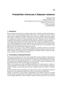
Knowledge discovery in database is defined as the nontrivial process of identifying valid, novel, potential useful and ultimately understandable patterns in data [FPS96]. In other words, it is to interpret and digest the large number of data of finding useful patterns and knowledge. Figure1.1 is an overview of the steps composing the KDD process [FPS96].
Figure 1.1: An Overview of the Steps Composing the KDD process [FPS96].
Figure 1.1 has a mistake: the output of the first action “selection” should be “Target data” instead of “Target Date”. I still keep the original figure because it is hard and time-consuming to reproduce a new and correct one. Based on figure 1.1, Fayyad et al. have outlined nine basic steps in [FPS96]: (1) Develop and understanding of the application domain and the relevant prior knowledge and identify the goal of the KDD process from the customer’s perspective. (2) Create a target data set by selecting a data set or focusing on a subset of variables or data samples on which KDD is to be performed.
5
(3) Data cleaning and preprocessing: do some basic operations including removing noise, collecting the necessary information to model or account for noise, deciding on strategies for handling missing data fields. (4) Data reduction and projection: find useful features to represent the data depending on the goal of the task. With dimensionality reduction or transformation methods, the effective number of variables under consideration can be reduced, or invariant representations for the data can be found. (5) Matching the goals of the KDD process to a particular data-mining method like summarization, classification, regression, clustering and so on. (6) Exploratory analysis and model & hypothesis selection: choose the data mining algorithms and select methods to search for data patterns which might be appropriate and matching a particular data-mining method with the overall criteria of the KDD process. (7) Data mining: searching for patterns of interest in a particular representational form or a set of such representations, including classification rules or trees, regression, and clustering. (8) Interpretation of mined patterns. User might return to step 1 to step 7 if the mined patterns do not match their particular goals. Visualization can be used in this step visualize the mined patterns and data in the extracted models. (9) The last step is to use the knowledge extracted directly, to incorporate them into another system for further actions, or to simply document it and report it to third parties.
From the above steps and figure 1.1, we can see that the KDD process is highly interactive with users and can contain loops between step eight and any other step from step one to step seven. Also, Fayyad et al. hold the view that KDD is an overall process including data mining as just one step in it [FPS96]. This is different with the traditional opinions which regard KDD as just another name of data mining and I think Fayyad et al.’s idea tells the differences between KDD and data mining and more systematic.
KDD has various successful applications in both science and business. In [FPS96], it also shows a lot of examples such as SKICAT, a system used by astronomers to perform image 6
analysis, classification, and cataloging of sky objects from sky-survey images; and ADVANCED SCOUT, a specialized data-mining system that helps National Basketball Association (NBA) coaches organize and interpret data from NBA games. All these applications have some features in common: the system deals with massive volumes of data of varieties of types and attributes and extracts understandable and useful knowledge from those data. There might be someone doubting that the data ADVANCED SCOUT deals with are not that much. However, this is really the case. According to [BCP97], in addition to the trivial game statistics, the collected NBA data include who took a shot, the type of shot, the outcome, any rebounds, etc. Each action is associated with a time code. Try to imagine, there are at least 48 minutes for a game and each game will play at least 82 games per season and how many shots in each game. The data can be recognized massive and ADVANCED SCOUT also shows its successful applications.
1.2.2
Decision Support (DS) and Decision Support Systems (DSS)
The term Decision Support (DS) is often used in various contexts related to decision making. However, unfortunately, although “Decision Support” seems rather intuitive and simple, there is no unified definition for it. However, M. Bohanec has provided some related definitions in [Boh01].
First of all, Decision Support (DS) is a part of decision making processes. A decision is the choice of one among a number of alternatives while decision making refers to the whole process of making the choice including the following steps: z
assessing problem
z
collecting and verifying information
z
identifying alternatives
z
anticipating consequences of decisions
z
making the choice using sound and logical judgment based on available information
z
informing others of decision
z
evaluating decisions 7
Also, the term “decision support” contains the word “support”, which means to support people in making decisions. Therefore, DS is concerned with human decision making [Boh01].
As illustrated in [Power97], Decision Support Systems (DSS) are defined as interactive computer-based systems intended to help decision makers utilize data and models in order to identify and solve problems and make decisions. Their major characteristics are: z
Decision Support Systems incorporate both data and models;
z
They are designed to assist managers in semi-structured or unstructured decision-making process, where unstructured and semi-structured mean the goals and objectives are not completely defined;
z
Decision Support Systems support, rather than replace managerial judgment.
Decision Support Systems can help structure decision processes and support analysis of the consequences of possible decision choices by making data easily accessible and allowing “what-if” analyses [Cai01].
Using the scope as criterion, D. J. Power has classified Decision Support Systems into two main categories in [Pow97]: z
Enterprise-wide DSS: linked to large data warehouses and serves many managers in the company;
z
Desktop, single-user DSS: a small system that runs on an individual manager’s PC.
More recently, many software packages have been produced which allow non-specialists to construct Decision Support Systems for themselves. These are called DSS generators, and Bayesian Networks software packages can be considered to be among them [Cai01]. Besides Bayesian Networks software packages, there are also other packages using different underlying techniques like: Influence diagrams, Decision trees, Mathematical modeling, Multi-criteria analysis, and Spreadsheets etc. Jeremy Cain provides more details for these techniques in [Cai01]. Here, I will just concentrate on how to use Bayesian networks to build a Decision Support System with a moderate size between Enterprise-wide and desktop DSS. 8
1.2.3
Knowledge Discovery and Decision Support in Land Planning
Land planning is a complex process including many steps. The complete steps are provided in [FAOUN] shown by figure 1.2.
Figure 1.2: The complete work flow for land planning. The first step can be further divided into sub tasks shown in figure 1.3.
Figure 1.3: The sub tasks for step 1 of land planning. In step 1, Knowledge Discovery (KD) can be applied to acquire information and knowledge
9
of related data resources and relevant experts. Decision Support (DS) can be applied to step 5 through step 7. Therefore, land planning is a test bed combining both Knowledge Discovery (KD) and Decision Support (DS). The problem is now how to integrate them together and this problem reminds us of Bayesian Networks.
1.2.4
An overview of Bayesian Networks
Bayesian Networks are composed of three components: z
Nodes: these nodes represent factors in an application domain. For example, a node called “Visit to Asia” means whether a patient has ever been to Asia. This node will perform as a factor in a diagnose domain. Each node has a finite set of mutually exclusive states. The factors can either be discrete or continuous. For instance, discrete factor can be whether a patient has even been to Asian and continuous factor can be rainfall depth. Both discrete and continuous factors have to be guaranteed to have a finite set of states. Factors are also often called variables.
z
Links: each link represents causal relationships between two nodes. Each link has a direction from cause to effect.
z
Conditional Probability Tables (CPTs): a set of probabilities which can be represented in tables. These probabilities specify the belief that a node would be in a particular state given the states of those nodes that affect it directly. If there are no nodes affecting it, its CPT just specifies its own probability distribution.
The first two components can be combined as the structure of Bayesian Networks while the third element is often called the parameters of Bayesian Networks.
Here is an example of Bayesian Networks named “Inheritance of eye colors”. This example is taken from [Ben99]. It is well known that eye colors are inherited from parents. We assume that there exist only two eye colors: blue and brown. The eye color of a person is fully determined by two alleles. One of these two alleles is from mother and the other is from father and each allele can either be type b or B, which are coding for blue eye color and brown eye color respectively. 10
Therefore, there are four types of combination: bb, bB, Bb, and BB among which only bb will produce blue eye color while the other three will produce brown eye color. Based on the above assumption, we can build the Bayesian Network as shown in figure 1.3.
Figure 1.3: The structure of the sample Bayesian Networks.
The structure has shown three nodes (variables) and two links. A complete Bayesian Network still needs to be configured with CPTs. The CPTs for this Bayesian Network can be shown in table 1.1. Xmother \ Xfather
bb
bB
BB
bb
(1,0,0)
(0.5,0.5,0)
(0,1,0)
bB
(0.5,0.5,0)
(0.25,0.5,0.25)
(0,0.5,0.5)
BB
(0,1,0)
(0,0.5,0.5)
(0,0,1)
Table 1.1: the CPTs for the sample Bayesian Networks
Table 1.1 shows the parameter of the sample Bayesian Network. The values in the circle brackets are illustrated as following: for example (1, 0, 0), which from mother bb and father bb means if the one’s parents both have blue eyes, the one will definitely has blue eyes. (0.5, 0.5, 0), which from mother bB and father bb means if the one’s mother has brown eyes and father has blue eyes, the one has equal chance to have blue eyes and brown eyes.
As we can see from this example, Bayesian Networks are graphical representations about an application domain composed with nodes, links and conditional probability tables. Bayesian Networks have answered the question: if event X happens with probability P ( X ) , what is the
11
probability that another event Y happens. Bayesian Networks solve this problem by its inference engine with proper inference algorithms, which will be illustrated in chapter 2. Given these features, Bayesian Networks are quite fit to help decision makers to make decisions by comprehensively evaluating those decisions in different scenarios.
Bayes Lab has listed a lot of examples in [BLA] like mining the customer database, health trajectory analysis, global risk analysis & security analysis, fraud detection and text mining. Details can be found in [BLA] which will not be outlined here. K. Sivakumar et al. have used Bayesian Networks as knowledge discovery means from distributed and heterogeneous databases to select relational models in [SCK03]. Also, [NS99] shows that Bayesian Networks can be applied to decision support area to combine multiple sources of data to support decision making. In a word, Bayesian Networks are techniques which can be used for both knowledge discovery and decision support.
This is the case in this project. The following section will introduce how Bayesian Networks work with the other techniques.
1.3
The Big Picture of This Project
In the context of land planning, the raw data are from various spatial databases containing different values of a suburb like rainfall depth, soil parameters, etc and other types of databases including other information. Apart from the spatial data, mankind knowledge and other factors like social, political issues are also needed to be considered. Figure 1.4 shows an overview of what is going on in this project.
As we can see from figure 1.4, KD techniques including Bayesian Networks are used to mining patterns / models that match our particular interest from spatial databases and other databases. These two procedures are subjective to the KD process mentioned in section 1.2.1 and they can contain loops, which indicate that re-mine the databases to get better patterns and models. Given
12
the patterns and certain expert knowledge, we use Bayesian Network to integrate them together and the output of this integration is our final product: the intelligent decision support system.
Figure 1.4: the big picture of this project.
The details of the database, expert knowledge are not available now because the project will actually start from March, 2007. But after meeting with ACT-PLA, we agreed to get them ready in the Project requirements which will be finished next semester (March, 2007 – June, 2007).
13
Chapter 2
Literature Review This chapter is the literature review concerning the KD techniques which will be used in our project. As discussed with Dr. Nianjun Liu, Bayesian Networks will be the main part coupled with a brief introduction of another technique, decision trees.
2.1
Decision Trees
A decision tree is a tree composed of three basic elements [ABE04], [Nil96]: z
A decision node, the internal node which specifies a test over one or more attribute;
z
An edge or a branch, which is directed, specifies the outcomes of the corresponding test;
z
A leaf, which is the leaf node of the tree, specifies the class the object being tested belongs to.
Figure 2.1 shows an example of a decision tree from [Nil96]. In figure 2.1, the internal nodes and the root node denoted by Ti are decision nodes doing testing over one or more attributes, and the braches specifies the outcomes of the tests while the leaves shows classes (denoted by number 1, 2 and 3) of the objects tested.
The technique for inducing a decision tree from given dataset is called decision trees or decision tree learning. This technique is being used in a wide range of areas including pattern recognition, data mining, machine learning, and decision support systems. It might be used in my project to cooperate building the Decision Support System.
Decision trees include two main phases [ABE04]: 14
z
Building the tree, a decision tree can be built based on a given training data set through selecting for each decision node the proper test attribute and defining the class for each leaf;
z
Classification, after the decision tree is built, it can be used to classify a new object instance by testing from the root node to a specific leaf.
Figure 2.1: A sample decision tree [Nil96].
These two phases involves several algorithms. Quinlan has developed the ID3 and C4.5 algorithms to construct the decision tree in [Qui93]. These two algorithms are the most popular ones and contain the following three procedures [ABE04]: z
The attribute selection measure: to select the best attribute (attributes) with the most discriminative power in order to classify the objects.
z
The partitioning procedure: according to the attribute (attributes) selected from the above procedure, this procedure will divide the training set objects into different classes.
z
The stopping judge: this procedure will check the conditions of completing building the decision tree.
[Quin93] has provided the details of the algorithms, which will not be completely covered in this report.
Although most of decision tree software is commercialized, it is not that hard to develop. We 15
might write our own decision components in our decision support system based on the algorithms mentioned above.
2.2
Bayesian Networks Principles
2.2.1
Essential Graph Theories and Definitions
Bayesian Networks are closely related to graph theory. The following section will use some useful terms from graph theory. It is necessary to make the definitions first. These definitions are taken from [Lau96].
Graph
A graph G = (V , E ) consists of a set of nodes, V and a set of edges E . An undirected edge u − v has both
(u, v ) ∈ E
and (v, u ) ∈ E . A directed edge
u → v only has (u , v ) ∈ E . Several terms related to the graph are defined as following: Parents of node v : pa (v ) = {u ∈ V | (u , v ) ∈ E I (v, u ) ∉ E} Children of node u : ch(u ) = {v ∈ V | (u , v ) ∈ E I (v, u ) ∉ E} Neighbours of node u : ne(u ) = {v ∈ V | (u , v ) ∈ E U (v, u ) ∈ E} Family of node u : fa (u ) = {u} U pa (a ) Path and Cycle A path of length l from a node u to a node v is a sequence
v0 , v1 ,⋅ ⋅ ⋅, vl of
nodes such that u = v0 and v = vl . A cycle is a path p = v 0 , v1 ,⋅ ⋅ ⋅, vl where v0 = vl . Direct Acyclic Graph, singly-connected Direct Acyclic Graph, and multiply-connected Direct Acyclic Graph A directed acyclic graph is a directed graph without any cycles. If the directions of all edges are removed and the resulting graph becomes a tree, then the DAG is 16
called singly-connected DAG. Otherwise, the DAG is a multiply-connected DAG. Moral graph and Triangulated graph If, in a DAG, edges between all parents with a common child are added and then the directions of all other edges are removed, the resulting graph is called a moral graph. A triangulated graph is an undirected graph where cycles of length three or more always have a chord, which is an edge joining two non-consecutive nodes. Clusters and Cliques A cluster is simply a subset of nodes in a graph. If all nodes in a graph are neighbours with each other, then the graph is called complete. A clique is a maximal set of nodes that are all pair wise connected.
2.2.2
Basic Ideas of Bayesian Networks
A Bayesian network is often referred as a Bayesian belief network or just belief network. As mentioned in the introduction part, a Bayesian network is a form of probabilistic graphical model, which, in probability theory and statistics, represents dependencies among random variables by a graph in which each random variable is a node, and edges between the nodes represent conditional dependencies [Mur98]. There are two types of graphical models, one is undirected graphical model also called Markov Random Field (MRFs) and the other one is directed acyclic graph (DAG) model. A Bayesian network is in the form of the latter one: a directed acyclic graph G = (V , E ) [Jen01]. In G = (V , E ) , G stands for the graph; V is the set of nodes; and E is the set of edges linking the nodes in V .
The chapter 1 of [Jen01] has illustrated the fundamental principles involved in a Bayesian Network. Here is a summation with essential probability calculus and mathematical proof in Appendix B. 1. In figure 2.1, A and B are both variables. Each node i ∈ V corresponds to a random variable X i with a finite set of mutually exclusive states. 2. Since a Bayesian Network is structured as a directed graph, there must be directed 17
edges linking different nodes such as figure 2.2.
Figure 2.2 Simple sample of two linked nodes in a DAG If there is a link from node A to node B, then, B is a child of A and A is a parent of B. The direction of the edge from A to B means A has an influence on B. pa (i ) denotes the set of parents of node i in graph G 3. A
directed
acyclic
graph
(DAG)
means
there
is
no
directed
path
A1 → A2 → ⋅ ⋅ ⋅ → An where A1 = An . 4. To
each
node i ∈ V
( ( )
table P X i | X j
j∈ pa (i )
).
,
there
is
attached
a
conditional
probability
5. From 3, the DAG also implies conditional independency relations between ( X i )i∈V . And using d-separation [Jen01] can be used to read the conditional independency relations from the DAG. More about d-separation will be in Appendix B. 6. Using the chain rule [Appendix B] we have that:
P (( X i )i∈V ) = ∏ P( X i | X i −1 ,..., X 1 ) .
(1)
i∈V
And a BN also implies that, each node is conditionally independent of all its non-descendants in the DAG given the value of all its parents. Based on this lemma, we have:
(
)
P (( X i )i∈V ) = ∏ P X i | (X j ) j∈ pa (i ) . i∈V
(2)
And this is the key point: the joint probability distribution represented by the Bayesian Network also called the Chain Rule for Bayesian Network. (Probability foundations and mathematical proofs for this sub-section is in Appendix B) For example: a BN is shown in figure 2.3.
18
Figure 2.3: A sample Bayesian Network. Then,
P( X 1 ,......, X 9 ) = P( X 9 | X 8 ,..., X 1 ) ⋅ P( X 8 | X 7 ,..., X 1 ) ⋅ ... ⋅ P( X 2 | X 1 ) ⋅ P( X 1 )
= P( X 9 | X 6 ) ⋅ P( X 8 | X 7 , X 6 ) ⋅ P( X 7 | X 5 ) ⋅ P( X 6 | X 4 , X 3 ) ⋅ P( X 5 | X 1 ) ⋅ P( X 4 | X 2 )
⋅ P( X 3 | X 1 ) ⋅ P( X 2 ) ⋅ P( X 1 )
2.2.3
Inferences in Bayesian Networks
In this part, it is assumed that nodes in Bayesian Networks represent discrete variables and node and variable might be used in different context but with the same meaning.
We can see from the previous sections of this report that a Bayesian Network can be constructed given the prior probability of the root nodes and the conditional probability of other nodes. The very original Bayesian Network represents our prior belief about the application domain. We might receive new information about the domain later and the new information which is formally known as evidence will affect our belief about the world to a certain extent. The process of updating probability of target variables given observed evidence is called inference in Bayesian Network.
The evidence is also called finding sometimes. Evidence on a variable is a statement of certainties of its states. If we can decide exactly which state the variable is in from the evidence, the evidence is called hard evidence. Otherwise, it is called soft evidence. 19
A Bayesian Network specifies a complete joint probability distribution (JPD) over all the variables. The JPD can also be obtained by combining or marginalizing the conditional probability tables (CPTs). Given the JPD, we can answer all possible inference queries by marginalization, as illustrated in [Mur98]. However, if each variable just has m states, the JPD will have the
( ) , in which
size O m
n
n is the number of variables. Therefore, summing over the JPD takes
exponential time. Some researchers have proposed some approximation inference algorithms like Monte Carlo method, to reduce the computation complexity. However, approximation inference algorithms are out of scope of this project and only exact inference algorithms will be covered in this section. Three exact inference algorithms will be illustrated here: Variable Elimination algorithms, Belief Propagation algorithms and Junction tree algorithms. Also, for better understanding the three algorithms, I have applied them to concrete examples respectively and the results are in Appendix C.
Variable Elimination
The basic principle of this method is to distribute sums over products as briefly illustrated in [Mur98]. But here, I will cover a general variable elimination method called Bucket Elimination for calculating marginal that works for any directed distribution including multiply connected graphs. The details of this method are provided in [Bar06]. Figure 2.4 provides a concrete example to help the illustration.
Figure 2.4: A simple Bayesian Network for illustration of Bucket Elimination.
The BN presents the distribution: 20
P (a, b, c, d , e, f , g ) = P( f | d )P (g | d , e )P(c | a )P (d | a, b) P (a )P (b )P(e ) . Now, for simplicity, we only consider calculating marginal, for example P ( f ) :
P( f ) =
∑ P(a, b, c, d , e, f , g ) = ∑ P( f | d )P(g | d , e)P(c | a )P(d | a, b) P(a )P(b)P(e)
a ,b , c , d , e , g
a ,b , c , d , e , g
We can distribute the summation over the various terms as follows:
P( f ) =
⎛
⎞⎛
⎞⎛
⎞
∑ P( f | d )P(a )⎜⎝ ∑ P(d | a, b)P(b)⎟⎠⎜⎝ ∑ P(c | a )⎟⎠⎜⎝ ∑ P(g | d , e)P(e)⎟⎠
a ,d , g
b
c
e
For convenience, let’s write the terms in the brackets as
∑ P(d | a, b )P(b) ≡ λ (a, d ) , B
b
∑ P(g | d , e)P(e) ≡ λ (d , g ) . E
e
The term
∑ P(c | a )
is equal to unity, and c is therefore eliminated directly. So,
c
P( f ) =
∑ P( f | d )P(a )λ (a, d )λ (d , g ) . B
E
a,d , g
Furthermore, we eliminate a and g . We can write:
⎞ ⎛ ⎞⎛ P ( f ) = ∑ P( f | d )⎜ ∑ P (a )λ B (a, d )⎟⎜⎜ ∑ λ E (d , g )⎟⎟ = ∑ P( f | d )λ A (d )λG (d ) . d ⎝ a ⎠⎝ g ⎠ d We illustrate this graphically in figure 2.5.
Figure 2.5: The bucket elimination algorithm applied to the BN in figure 2.3. It is a little tricky to read figure 2.5. The arrows specify the place where the eliminating output will go in each column. Each row shows the content associated with the variable which is about to be eliminated. For instance, the row of variable E is the content associated with E that is 21
about to be eliminated in the first place, and the output of this elimination is P ( g | d ) , which will be put in the row of variable G , which will be eliminated before variable D . This output will then be written as
λE (d , g ) in variable G ’s row to be eliminated. Each step of elimination will
reduce the height by one but increase the width by one. The following illustration is more formal.
Initially, we define an ordering of the variables, beginning with the one we wish to find the marginal for from the bottom to the up. In this case, the ordering is f , d , a, g , b, c, e . Then, starting with highest node e , we put all functions that mention e in the e bucket. Continuing with the next highest bucket c , we put all the remaining functions that mention c in this c bucket. Following this method, we can put the functions in the corresponding buckets. After eliminating the highest bucket e , we pass a message to node g . Immediately, we can also eliminate bucket c since this sums to unity. Also, following this method, we will finally get the target marginal.
We can also calculate the marginal for the other nodes using the same procedures. It is possible that we can always choose an ordering to eliminate the variables with the amount of computation scaling linearly with number of the variables in the graph [Bar06]. The Bucket Elimination procedure will also work on undirected graphs and multiple-connected directed graphs.
Belief Propagation (BP)
The Belief Propagation method was specifically illustrated in [Pea88], so it is sometimes also called Pearl’s BP algorithm. This report will only cover the Belief Propagation for singly-connected graph as a summary for the detailed illustration in [Bar06].
According to [Pea88], given a singly-connected Bayesian Network, we can define the belief of a node x in the following way with the help of figure 2.6.
22
Figure 2.6: A singly-connected Bayesian Network for illustration of basic idea of Belief Propagation Algorithm
Then,
Belief ( x ) = P( x | e ) = P(x | e + , e − )
(
) ( ( )
)
(
) (
P e − | x, e + • P x | e + P e− | x • P x | e+ = = P e− | e+ P e− | e+
(
)
)
= α • P(e − | x ) • P (x | e + )
α=
1 P e | e+
(
−
Because e
+
(4)
)
(5)
and e
−
are conditionally independent given x ,
α will be a positive constant
(
−
value. So belief of variable x will be positive proportional to the product of P e | x
(
and P x | e
+
)
). This is the motivation of the BP algorithm. In the rest part of this method,
P (e − | x ) will be called as λ messages coming from children of variable x and P (x | e + ) will be called as
ρ messages coming from parents of variable x .
It is much easier to analyze the Belief Propagation algorithm using a concrete singly-connected Bayesian Network as shown in figure 2.7.
23
Figure 2.7: A singly-connected Bayesian Network for illustrating Belief Propagation Algorithm.
The BN in figure 2.6 represents distributions:
P(a, b, c, d , e, f , g ) = P(d | a, b, c )P(a )P(b )P(c )P(e | d )P( f | d )P( g | d ) . Consider calculating the marginal p (d ) , which is summing the joint distribution over the remaining variables a, b, c, e, f , g as following:
P(d ) = ∑ P(d | a, b, c )P(a )P(b )P(c )∑ P(e | d )∑ P( f | d )∑ P( g | d ) . abc
e
f
(6)
g
In the above equation, we will define two different types of messages as following:
ρ a − > d (a ) = P(a ) ; ρ b −> d (b ) = P(b ) ; ρ c − > d (c ) = P(c ) ; λe −> d (d ) = ∑ P(e | d ) ; e
λ f − > d (d ) = ∑ P( f | d ) ; f
λ g −> d (d ) = ∑ P( g | d ) . g
In the above equations, and
λ messages contain information passing up from children of node d ,
ρ messages contain information passing down from parents of the same node.
Therefore, equation (6) can be rewritten as:
P(d ) = ∑ P(d | a, b, c )ρ a − > d (a )ρ b −> d (b )ρ c − > d (c )λe − > d (e )λ f − > d ( f )λ g −> d ( g )
(7)
abc
Furthermore, consider some further modification on the original BN as shown in figure 2.8. 24
Figure 2.8: The BN after some modification of node A (a parent of node D) and node G (a child of node D).
Compared to the original BN, the only messages need to be adjusted for marginal p (d ) are those from a to d , namely
ρ a − >d (a ) and from g to d , namely ρ g − > d (d ) . There will be no
need to change the form of equation (7). We only need to change the content of
ρ a − >d (a ) and
λ g − > d (d ) as following: ρ a − > d (a ) = ∑ P(a | h, i )P(h )P(i )∑ P( j | a ) ; h ,i
j
λ g − > d (d ) = ∑ P( g | o, d )P(o )∑ P(m | g )∑ P(n | g ) , g ,o
m
n
And the content of the above two equations can be rewritten using the form of
ρ messages and
λ messages as following:
ρ a − > d (a ) = ∑ P(a | h, i )ρ h − > a (h )ρ i − > a (i )λ j −> a (a ) ; h ,i
λ g − > d (d ) = ∑ P(g | o, d )ρ o − > g (o )λ m − > g ( g )λn − > g ( g ) . g ,o
From the illustration above, we can see that to pass a message from a node a to a child node b , we need to take into account information from all the parents of a and all the children of a , except b . Similarly, to pass a message from node b to a parent node of a , we need to gather information from all the children of node b and all parents of b , except a .
25
After the analysis of the concrete example, we can generalize the Belief Propagation Algorithm, which will be given as following.
A general node d has messages coming from its parents and children, and we can collect all the messages from its parents that will then be sent through d to any subsequent children as:
ρ d (d ) =
∑ P(d | pa(d )) ∏( ρ) (i ) . i ,d
pa ( d )
i∈ pa d
Similarly, we can collect all the information coming from the children of node d that can subsequently be passed to any parents of d as:
λd (d ) =
∏ λ (d ) .
i∈ch ( d )
i ,d
The messages collected will be used in the following message calculation.
[Message Definition] The messages are defined as:
λc ,a (a ) = ∑ λc (c )
∑
i∈ pa (c )\ a
c
ρ b ,d (b ) = ρ b (b )
P (c | pa (c ))
∏ ρ (i ) ,
i∈ pa (c )\ a
i ,c
∏ λ (b) .
i∈ch (b )\ d
i ,b
[Initialization] (1) For every evidential node i , set z
ρ i (i ) = 1 for node i in the evidential state, ρ i (i ) = 0 otherwise.
z
λi (i ) = 1 for node i in the evidential state, λi (i ) = 0 otherwise.
(2) For every non-evidential node i with no parents, set
ρ i (i ) = p(i ).
(3) For every non-evidential node i with no children, set λi (i ) = 1 . [Iteration] For every non-evidential node i we then iterate: 26
(1) If i has received the
ρ messages from all its parents, calculate ρ i (i ) .
(2) If i has received the
λ messages from all its children, calculate λi (i ) .
(3) If
ρ i (i ) has been calculated, then for every child j of i such that i has received the
λ messages from all its other children, calculate and send the message ρ i, j (i ) . (4) If
λi (i ) has been calculated, then for every parent j of i such that i has received the
ρ messages from all of its other parents, calculate and send the message λi, j ( j ) .
[Get the Result] Repeat the above (1) – (4) until all
λ and ρ messages between any two adjacent nodes have
been calculated. For every non-evidential node i , compute
ρ i (i )λi (i ) . The marginal
P (i | evidence) is then found by normalizing this value.
The complexity of Belief Propagation Algorithm is time exponential in the maximum family size and linear in space. The Belief Propagation Algorithm is most used for exact inference for singly-connected Bayesian Network.
Recent
research
applies
this
algorithm
for
approximation
inference
for
multiply-connected Bayesian Network. But this is out of the scope of this report.
The Junction Tree Algorithm (JTA)
The problem of conditioning Bayesian Networks on observations is in general NP-hard, but experience shows that in many real systems the networks are sparsely connected and therefore the calculations are tractable [Rip96]. The Bucket Elimination method and Belief Propagation Method are both proposed in this case. The Bucket Elimination method can generally answer any queries for both singly-connected BNs and multiply-connected BNs, but it is not efficient enough due to re-calculating for new queries. The Belief Propagation method avoid this re-calculating using dynamic programming, however, it encounters problems when there are loops in the BN [Mur98]. 27
Therefore, many algorithms have been proposed and the Junction Tree Algorithm is a popular one that can conquer the drawbacks in the Bucket Elimination method and Belief Propagation method using a new data structure called the junction tree.
The Junction Tree Algorithm was designed by the Odin group at Aarhus University [Jen94]. Unlike the Belief Propagation Algorithm, the Junction Tree Algorithm can be applied to any Bayesian Networks.
Since the Junction Tree Algorithm is popular and also the underlying algorithm adopted in NETICA, it will be detailed illustrated in this section. All the algorithms in the following illustration originate from [Bar06] and [HD94], and the illustration itself is an integration of the original works from [Bar06] and [Ben99].
The Junction Tree Algorithm includes two main steps, transformation and propagation. The first step, transformation, builds an undirected junction tree from the original Bayesian Network. In most cases, this step is only carried out once. We then propagate received evidence and make inference about variables using only the junction tree from the first step in the second step, propagation.
Before giving the detailed algorithm, the essential terms and theories will be explained first.
Cluster Tree
Given a Bayesian Network G = (V , E ) , a cluster tree over V is a tree of clusters from V . The clusters are subsets of V such that their union is equal to V . The edges between the cluster in the tree is labeled with the intersection between two clusters A and B , and denoted by S AB = A I B . These intersections are defined as separator sets. Figure 2.9 shows an example of a cluster tree.
28
Figure 2.9: An example of a cluster tree, where clusters are displayed as ovals and the separators are displayed as squares.
Junction Tree Given a Bayesian Network G = (V , E ) , a junction tree over V is a cluster tree such that all nodes between any two pair of nodes A and B contains the intersection A I B . What should be noticed here is that the node in a cluster tree contains no longer just one variable but a cluster of variables. Figure 2.10 shows an example of a junction tree.
Figure 2.10: An example of a junction tree, where clusters are displayed as ovals and the separators are displayed as squares. The example shown in figure 2.9 is not a junction tree because the clusters and separator sets along the path between ade and cde do not contain their intersection de .
Decomposition and Triangulation Three joint subsets A , B and C of an undirected graph G = (V , E ) is said to 29
form a composition of G if: z
V = AU BUC
z
C separates A and B , and
z
C is a complete subset.
A graph that can be decomposed into cliques by decomposition is called a decomposable graph. And if an undirected graph is decomposable, it could also be triangulated.
Potential
A potential
φ A over a set of variables X A is a function that maps each
instantiation of variable x A from X A into a non-negative real number, denoted by φ A ( X A ) . There are two basic operations on potentials: marginalization and multiplication. Given two clusters of random variables where X A ⊆ X B . Then the marginalization of denoted by φ A =
∑φ
B
. Each
X A and
XB
φ B into X A is a potential φ A ,
φ A ( x A ) is computed as the sum
∑ φ (x , i ) B
B
i
XB \X A
where xB , i are all instantiations of X B such that they are consistent with x A . The multiplication of
φ A and φ B is a potential φC , where C = A U B , denoted
by φC = φ Aφ B . Each
φC ( xC ) is computed as the multiplication φ A (x A )φ B ( x B )
where both instantiation x A and instantiation x B are consistent with xC . Potentials are defined to denote the probability quantitatively from another perspective, and they do not need to sum to one.
Factorization of Potentials An undirected graph G is said to be an independent map of distribution if for any clusters A and B with separator C , variables in A are independent of variables B given all evidential variables in C. Then a probability distribution is said to be decomposable with respect to G if G is an independent map and triangulated.
30
Given a decomposable probability distribution P (V ) with respect to G , it can be written as the product of all potentials of the cliques divided by the product of all potentials on the separators, denoted by
∏φ P(V ) = ∏φ
C
C∈CS
(8) S
S ∈SS
In equation (8), CS is the set of all cliques, SS is the set of all separators and
φC is the potential over cluster C . This is key idea and motivation of the Junction Tree Algorithm.
The following section is the main course of the algorithm based on the definitions and theories given above.
Step 1) Transformation
In this step, we will create a new undirected graph from the original DAG of the Bayesian Network through the following algorithm.
[ALGORITHM JTA.T] 3.
Create a new undirected graph. This graph is the corresponding moral graph of the DAG of the Bayesian Network.
3.
Add edges to the moral graph to form a triangulated graph.
3.
Select cliques that are subsets of nodes in the triangulated graph.
3.
Using these cliques, create a junction tree by connecting the cliques with separator sets.
This algorithm is a general one describing the procedure of the transformation. Each step will be implemented by individual sub-algorithm respectively.
First of all, we need to create a new undirected graph, which is the moral graph of the DAG of the
31
Bayesian Network. This is done by ALGORITHM JTA.T.M. [ALGORITHM JTA.T.M] 2.
Create a copy G M of the original DAG G .
2.
For each node u , do for each pair of nodes in the parent set of u , pa (u ) add an undirected graph to G M .
2.
Make G M undirected by dropping the directions of all the edges.
Figure 2.11: The left one is the DAG of the Bayesian Network to be moralized. The right one is the moralized graph with dotted edges that are added during the moralization.
Figure 2.11 shows the moralization of a DAG of a Bayesian Network. The node b has two parents a and d unlinked, so an edge between a and d has to be added. The same thing is done to the parents of node f . The dotted edges shows are added during the moralization.
After we get the moralized graph, we need to triangulate it. An undirected graph is triangulated if all cycles of length larger than three has a chord, which is an edge joining two non-consecutive nodes. The process of triangulation is actually a process of eliminating nodes. An elimination of a node u is done by first connecting all of u ’s neighbours pair wise, and then remove u and all edges connected to it. This will be shown in figure 2.12. As shown in figure 2.12, node e is the one we want to eliminate. We first identify the induced cluster
{a, c, d , e}
and then connect e ’s
neighbours pair wise ( {a, c} and {a, d } ). Finally, the node e is eliminated together with its links with its neighbours.
32
Figure 2.12: An example of elimination of a node.
There are several triangulation algorithms. To find a best one is NP-hard [HD94, Jen94]. However there are many heuristic algorithms that produce at least close to optimal triangulation graphs. Here is the algorithm for triangulating any undirected graph from [HD94].
[ALGORITHM JTA.T.T] 1.
′ of G M from the moralization. Create a copy G M
1.
′ has nodes left As long as G M a)
′ that causes the least number of edges to be added if it is Select the node u from G M removed. If choice is between two or more nodes, select the one that induces the cluster (node u and all its neighbours) with the smallest weight (defined below).
a)
Connect all nodes in the cluster that is induced by selected node u . Add the corresponding edges to G M if they are new to G M .
1.
a)
Save each induced cluster that is NOT a subset of any precious saved cluster.
a)
′ . Remove u from G M
G M , with the additional edges added in step 2, is now triangulated.
The term mentioned in step 2a is defined: z
The weight of a node u is defined as the number of states the corresponding variable has, denoted by w(u ) .
z
The weight of a cluster is the product of the weight of its nodes, denoted
33
by w( A) =
∏ w(u ) . u∈ A
Now, we are in the position to build the junction tree. The vertices of the junction tree are the cliques saved during the triangulation. What we need to do is to connect these cliques so that it satisfies the junction tree definition. An approach from [HD94] is adopted here.
[ALGORITHM JTA.T.BJT] 1.
Two things need to be done: a)
Create a set of trees each containing a single clique. These cliques are the ones saved after triangulation. We assume that there are n cliques. Therefore, we will create a n tree forest.
a) 1.
1.
Create an empty set S to be used for storing separators.
For each distinct pair of cliques A and B : a)
Create a candidate separator, S AB containing the intersection A I B .
a)
Insert S AB into S .
Repeat until n − 1 separators have been inserted into the forest created in 1a. a)
Select and remove the separator S AB from S that has the largest mass (defined below). If two separators have equal mass, select the one with the smallest cost (defined below).
a)
If the clique A and B are on different trees in the forest, then join the two cliques inserting S AB between them.
1.
The forest contains of one tree, which is the junction tree.
The terms used in step3 are defined: z
The mass of a separator S AB , denoted by m(S AB ) , is the number of variables it contains.
z
The cost of a separator S AB , denoted by c(S AB ) = w( A) + w(B ) , where w( A) is the weight of the clique A .
We finally have got a junction tree, for easily understanding, a concrete example will be set up
34
here. This example is the one used in the previous section, namely “Asia”. Figure 2.13 shows the DAG of the Bayesian Network.
Figure 2.13: The DAG of the Bayesian Network of “Asia”.
Each node in the DAG shown in figure 2.12 has two states. Now we will work through this example for the transformation using the algorithms illustrated above.
Moralization
Figure 2.14: The moral graph after moralization.
35
Figure 2.14 shows the moral graph of the original DAG. In the following illustration, we use the upper-case letter in the bracket to denote each variable, e.g. “A” stands for “Visit to Asia?” etc. The dotted lines are added between the node sets {T, L} and {E, B} according to ALGORITHM JTA.T.M.
Figure 2.15: The triangulated graph of the moralized graph.
Triangulation
Figure 2.15 shows the triangulated graph of the moralized graph, where the added edge between L and B is dotted. Table 2.1 shows each step of the node elimination during the triangulation process.
Step
Eliminated Node
Edges Added
Induced Clusters
1
A
none
{A, T}
2
X
none
{X, E}
3
D
none
{D, B, E}
4
T
none
{T, E, L}
5
S
{B-L}
{S, B, L}
6
L
none
{E, B, L}
7
E
none
{E, B}
36
*
*
*
*
*
*
8
B
none
{B}
Table 2.1: The elimination ordering showing eliminated nodes, added edges and induced clusters. Those clusters marked with * are those saved for building a junction tree.
Building a junction tree
The saved clusters are {A, T}, {X, E}, {D, B, E}, {T, E, L}, {S, B, L}, and {E, B, L}. They will form the n-tree forest. It is also easy to find the separator set S : {T}, {E}, {B}, {L}, {E, B}, {E, L}, and {B, L}. According to ALGORITM JTA.T.BJT, we need to select five separators from S to connect the six clusters with respect the selecting rules.
Figure 2.16 shows the final production of the transformation procedure. What we finally got is the junction tree. The nodes displayed as oval are cliques and the nodes displayed as square are separators.
Figure 2.16: The junction tree of the original Bayesian Network.
All the above processes are graphical transformation. Apart from the graphical transformation to set up the junction tree, we still need to do the quantitative transformation. What we have to do is to initialize the junction tree by inserting the probability distribution into the junction tree properly.
37
[ALGORITHM JTA.T.IJT] 4.
For each cluster A and separator S AB , do the assignment:
φA ← 1 S AB ← 1 4.
For each node u in the original Bayesian Network DAG, assign u a cluster A that contains fa (u ) and call A the parent cluster of fa (u ) . Then include the conditional probability P (u | pa (u )) ( or just P (u ) if there are no parents) into
φ A according to
φ A ← φ A • P(u | pa(u ))
Now the transformation process has been finished. The following work is to do the information propagation.
Step 2) Information Propagation
After the junction tree is initialized, its potential does indeed satisfy the equation (8). But it might not be consistent. Recall when we assign the parent cluster to a specific node in the original DAG, there might be more than one parent clusters. In ALGORITHM JTA.T.IJT, the parent cluster is arbitrary assigned. For example, there are two cliques A and B , which are connected with a separator S AB , and both contain the variable u . Marginalization on both A and B to get P(u ) , might not give the same result. Then our job is to solve this problem to make the probability locally consistent as well as globally consistent. Technically, we have to keep equation (8) hold globally and locally.
First we will cover the message passing algorithm and then introduce the global propagation algorithm.
A single message passing between two clusters A and B are composed by two steps. The first
38
one, called projection, passes the message from A to the separator S AB . The second step, called absorption, passes the message from the separator S AB to B .
[ALGORITHM JTA.IP.MP] (PASS-MESSAGE (A, B)) 3.
Projection. Update the potential of the separator S AB :
φ Sold ← φ S AB
φS ← AB
AB
∑φ
A
A \ S AB
3.
Absorption. Update the potential of the receiving cluster
φ B ← φ BOld •
φB :
φS AB φ Sold AB
old If φ S AB = 0 , then φ B ← 0 .
[ALGORITHM JTA.IP.GP.1] Choose an arbitrary cluster A : 3.
Unmark all clusters. Call COLLECT-EVIDENCE (A, NIL) (defined below).
3.
Unmark all clusters. Call DISTRIBUTE-EVIDENCE (A) (defined below).
[ALGORITHM JTA.IP.GP.2] (COLLECT-EVIDENCE (A, C)) 2.
Mark A with a specific marker.
2.
While there are unmarked Bi ∈ ne( A) : Call COLLECT-EVIDENCE ( Bi , A)
2.
Call PASS-MESSAGE (A, C) back to the invoking cluster C if C ≠ NIL .
[ALGORITHM JTA.IP.GP.3] (DISTRIBUTE-EVIDENCE (A)) 4.
Mark A.
4.
While there are unmarked Bi ∈ ne( A) :
39
Call PASS-MESSAGE (A, Bi ) 3.
While there are unmarked Bi ∈ ne( A) : Call DISTRIBUTE-EVIDENCE ( Bi ).
The ALGORITHM JTA.IP.GP is a recursive algorithm. This makes itself run fast. After the global propagation, the whole junction tree will become consistent and associated with the joint probability distribution over clusters. If one wants to get the probability of one variable, he just needs to choose a cluster containing that variable and do marginalization to get the corresponding probability. The smaller the size of the chosen cluster is, the faster the calculation will be.
After the global propagation is finished, we actually just make the junction tree consistent for the prior probability distribution. If there are new evidences observed, we need to update the algorithm to insert the observations without invaliding the consistency.
As we are dealing with only the discrete variables other than continuous variables, we can introduce a new likelihood function to code evidence as following. The likelihood function of a variable u can be denoted as
λu (u ) = 1 , when u is in the observed state, 0 otherwise. When a variable is unobserved, we can set the likelihood function to a constant: λu (u ) =
1 , n
where n is the number of states of variable u .
We can insert the new observations at the initial stage as initialization. Therefore the initialization algorithm can be revised.
[ALGORITHM JTA.T.IJT.revised] 1.
For each cluster and separator A , do the assignment:
φA ← 1 2.
For each node u : 40
)
Assign to u a cluster A that contains
fa (u ) and call A the parent cluster
of fa (u ) . Then include the conditional probability P (u | pa (u )) (or just pa (u ) if there are no parents) into
φA :
φ A ← φ A • P(u | pa(u )) )
Set each likelihood function to one:
λu (u ) = 1 2.
For each observation u = u1 : )
Encode the observation as likelihood λu .
)
Identify a cluster A that contains u and update
new
φ A and λu as:
φ A ← φ A • λunew λu (u ) = λunew
And this initialization will drive the global propagation again with the new observed evidence. We will get the new probability distribution over clusters as well as new inference result based on new evidence. So far, we are really able to conduct posteriori inference. Appendix C has provided more concrete examples to walk through those three inference algorithms.
2.2.4
Learning of Bayesian Networks
The Bayesian Networks can be constructed manually in the general steps, which will be illustrated below. Also they can be constructed automatically by learning from the existing observed data or databases.
The latter method is called learning of Bayesian Networks. Like the construction manually, learning involves both the structure and parameters of each conditional probability distribution of each node, and both of them are possible learnt from data [Mur98].
41
The learning process is on the basis of the following four cases shown in table 2.2:
Case
Structure of BNs
Completeness of Data
Algorithms and Methods
1
Known
Complete
Maximum likelihood Estimation
2
Known
Partial
Expectation Maximization
3
Unknown
Complete
Search through model space
4
Unknown
Partial
Expectation Maximization & Search through model space
Table 2.2: The cases based on which learning of Bayesian Networks will be classified.
As shown in table 2.2, according to the nature of Bayesian Network structure and completeness of data, there are four cases. A known structure means the graphical topology of a Bayesian Network has already been given. A complete data/database means all the variables in that Bayesian Network are observed to be at certain states. Otherwise, the data/database is called partial observed, which also means there are some variables’ states are unknown.
This report will not detailed illustrate those methods and algorithms due to the complexity and existing controversies involved. The listed methods and algorithms are the ones with the widest recognition and popularity. Those methods and algorithms will be more deeply understood during next semester and will be covered in next semester’s report.
2.2.5
Software Toolkits for Bayesian Network
In table 2.3 and table 2.4, some software packages for Bayesian Networks / Graphical models will be introduced [Sof01, Sof02]. These software packages may apply in the project.
The meanings of the headers in the tables are explained as below: z
Name: The name of the software or software packages;
z
Web location: The website of the software or software packages;
z
Authors/Company:
The authors or company doing the development; 42
z
Free?: F means free (although possibly only for academic use) while $ stands for commercial software (although most have free or trial version restricted in various ways);
z
Comments: Special notes about the software or software packages;
z
Src: Whether the source code is included? N means no while if yes, the language used for developing is also provided, such as Java, Matlab, C/C++, Lisp, etc;
z
API: Whether application program interfaces are provided? N means the program cannot be integrated into you own code while Y means the other side;
z
Exec: The executable nature, which OS supported? W means Windows, U means Unix, M means Mac, and or- means any machine with a compiler;
z
D/C: Whether continuous-valued nodes supported. G means Gaussians nodes supported analytically, Cs means continuous nodes supported by sampling, Cd means continuous nodes supported by discretization, Cx means continuous nodes supported by some unspecified method, and D means only discrete nodes supported;
z
GUI: Whether a Graphical User Interface included. Y means yes while N means no;
z
Params: Whether parameter learning included. Y means yes while N means no;
z
Struct: Whether structure learning included. Y means yes while N means no;
z
D/N: Whether decision networks/influence diagrams supported. Y means yes while N means no;
z
D/U: What kinds of graphs are supported? U means only undirected graph, D means only directed graphs, UD means both undirected and directed and CG means chain graphs (mixed directed and undirected)
z
Inference: Which inference algorithm is used? JT means Junction Tree, VE means variable (bucket) elimination, E means Exact inference (unspecific), C means Markov chain Monte Carlo (MCMC), GS means Gibbs sampling, IS means Importance sampling, S means sampling, O means Other, ++ means Many methods provided, ? means Not specified, N means None, the program is only designed for structure learning from completely observed data.
43
Name
Web location
Author/Corp.
Bayda
http://www.cs.helsinki.fi/research/cosco U. Helsinki /Projects/NONE/SW/
BayesiaLab http://www.bayesia.com/
Bayesware Discoverer
Bayesia Ltd
Free? Comments F
Bayesian Naive Bayes classifier.
$
Structural learning, adaptive questionnaires, dynamic models
$
Uses bound and collapse for learning with missing data.
http://www.bayesware.com/
Bayesware
BNT
http://www.cs.ubc.ca/~murphyk /Bayes/bnt.html
Murphy (U.C.Berkele F y)
Also handles dynamic models, like HMMs and Kalman filters.
BNJ
http://bnj.sourceforge.net/
Hsu (Kansas) F
-
Business http://www.data-digest.com/ Navigator 5
Data Digest Corp
-
http://www.math.auc.dk/~jhb CoCo+Xlisp /CoCo/information.html
Badsberg (U. F Aalborg)
$
Designed for contingency tables.
GDAGsim
http://www.staff.ncl.ac.uk/d.j.wilkinson Wilkinson (U. F /software/gdagsim/ Newcastle)
Bayesian analysis of large linear Gaussian directed models.
Genie
http://www2.sis.pitt.edu/~genie/
U. Pittsburgh F
-
GMRFsim
http://www.math.ntnu.no/~hrue /GMRFsim/
Rue (U. Trondheim)
F
Bayesian analysis of large linear Gaussian undirected models.
Java Bayes
http://www2.cs.cmu.edu/~javabayes /Home/
Cozman (CMU)
F
-
MSBNx
http://research.microsoft.com/adapt /MSBNx/
Microsoft
F
-
Netica
http://www.norsys.com/
Norsys
$
-
Vibes
http://johnwinn.org/
Winn & Bishop (U. Cambridge)
F
Not yet available.
44
Web Weaver
Xiang (U.Regina)
http://snowhite.cis.uoguelph.ca /faculty_info/yxiang/ww3/ Table 2.3:
F
-
Software packages’ name, web location and developers
Name
Src
API
Exec D/C GUI Params Struct D/N D/U Inference
Bayda
Java
Y
WUM G
BayesiaLab
N
N
-
Bayesware Discoverer N
N
Y
Y
N
N
D
?
Cd Y
Y
Y
N
CG JT,G
WUM Cd Y
Y
Y
N
D
?
BNT
Matlab/C Y
WUM G
N
Y
Y
Y
D,U S,E(++)
BNJ
Java
-
-
D
Y
N
Y
N
D
JT, IS
Business Navigator 5 N
N
W
Cd Y
Y
Y
N
D
JT
CoCo+Xlisp
C/lisp
Y
U
D
Y
Y
CI
N
U
JT
GDAGsim
C
Y
WUM G
N
N
N
N
D
E
Genie
N
WU
WU
D
W
N
N
Y
D
JT
GMRFsim
C
Y
WUM G
N
N
N
N
U
MC
Java Bayes
Java
Y
WUM D
Y
N
N
Y
D
VE, JT
MSBNx
N
Y
W
D
W
N
N
Y
D
JT
Netica
N
WUM W
G
W
Y
N
Y
D
JT
Vibes
Java
Y
WU
Cx Y
Y
N
N
D
V?
Web Weaver
Java
Y
WUM D
N
N
Y
D
?
Table 2.4:
Y
Features comparison of software packages
As discussed with Dr. Nianjun Liu, we might use Netica very often in the future wok. NETICA’s features have already been included in table 2.3 and table 2.4. I personally think that the Java APIs provided by Norsys are the most attractive parts of NETICA. We might use these APIs in our own decision support system.
2.3
Previous Applications of Bayesian Networks in Land Planning
2.3.1
General Steps for using Bayesian Networks in Land Planning
45
Although [Cai01] is a paper of guidelines for using Bayesian Networks to support the planning and management of development programs in the water sector, the general ideas can be extracted and applied to other sectors including land planning. The following steps are just summarized from [Cai01].
Step 1: Be clear about what you want to use the Bayesian Network for
During this step, the designers should identify the objectives of the management (in this case, land planning) and also define the criteria on which the decisions about which options to choose will be based on. In addition, the designers should be aware of the management interventions they wish to investigate as a way of achieving their objectives.
Apart from the above, the designers should also identify the groups of people involved in the management process.
Step 2: Establish contracts with stakeholders
After identifying groups of stakeholders in Step 1, the designers should classify them by their different importance to the project. Also they have to decide how many representatives for each group to be directly involved in the process of building the DSS. The number of people will be dependent on the time and resources they have available. But in all cases, stakeholder group representatives should meet the following criteria: z
They must be accepted by the stakeholder group which they are representing;
z
They should possess good local knowledge;
z
They are available for consultation and able to attend all the workshops.
Step 3: Initial stakeholder group consultation
46
Carry out the discussions with each group of representatives in turn. Begin with explaining what you are trying to do (the objectives of the project and criteria, etc). Ask them to comment on your objectives from the perspective of their own group. Sample questions like: z
Do they think that achieving these objectives is important?
z
What other objectives do they think are important as well?
Given these responses, you might need to revise your original objectives until they reach a certain level of agreement among the representatives.
Next, ask them to describe the ways in which they think the agreed objectives can be achieved. You would better gain enough information to complete Step 4 by thinking in terms of “cause and effect”. Recording the discussion, if possible, will be useful to take notes of the questions and answers.
Step 4: Construct preliminary Bayesian Networks
In this step, you shall transfer the information captured in the previous step into the form of a Bayesian Network diagram. This should be done for each stakeholder group and will allow you to communicate it to others more easily.
Jeremy Cain has provided a general network structure with different groups of variables (nodes). Tests show it will be easier to build a Bayesian Network if you do this. The general network structure can be shown as figure 2.18.
47
Figure 2.18: the general network structure. Those terms in figure 2.18 can be explained in table 2.5.
Terms
Description
Objectives
The things you wish to achieve by the management (land planning). These maybe things you wish to prevent from worsening. They will define the criteria on which your management choice will be based.
Interventions
The things you wish to implement in order to achieve your objectives. They can also be thought of as management options.
Intermediate factors
Factors which link objectives and interventions
Controlling factors
Factors which cannot be changed by intervening at the scale you are considering but control the environmental systems at that scale, in some way. Such as: population, rainfall, and government policies, etc.
Implementation factors
Factors which directly affect whether the intervention can be successfully implemented both immediately and in the future (depending on whether the intervention is implemented as a one-off or over a longer period)
Additional impacts
Factors which are changed as a result of interventions that do nor affect anything else in the environmental system Table 2.5: Explanations to the terms from figure 2.17.
The arrows in figure 2.17 show how the categories are likely to be linked. However, figure 2.17 just shows a suggestive example, not for every case.
When the designers think they have finished, they have to check that the Bayesian Network is logical and complete according to the guidelines listed in [Cai01].
48
Step 5: Further stakeholder group consultation
Arrange a meeting with each stakeholder group separately for the following objectives: z
To check the validity of the relationships deduced from Step 3 and include in the preliminary Bayesian Network constructed in Step 4;
z
To define the states for each node.
Any changes suggested by the stakeholder group should be accepted and the preliminary Bayesian Network diagram changed accordingly. Once the stakeholders are satisfied with the Bayesian Network diagram, it has to be reviewed again to make sure the links in the preliminary Bayesian Network build in Step 4 properly represent how the stakeholders see the variables working together.
Step 6: Draw conclusions from stakeholder consultation
Following completion of Step 5, a Bayesian Network diagram accurately representing the perceptions of each stakeholder group will be constructed. Therefore, it is possible to use the diagrams to identify: z
Potential issues of consensus between groups;
z
Potential issues of conflict between groups.
When these issues have been identified, a stakeholder workshop shall be held to find out the reasons for them.
Step 7: Hold joint stakeholder workshop to discuss differences in viewpoints
The objective of this workshop is to allow different stakeholder groups to discuss the reasons for any differences in the interventions they favour. All stakeholder groups should be present at this workshop so that they can discuss the issues together. Finally, we will get possible compromises and make a final decision among those possibilities. 49
Step 8: Complete stakeholder Bayesian Networks
The Bayesian Networks shall be altered again according to the conclusions gained in Step 7. Generally doing this will involve adding and deleting nodes and links appropriately. Notice that, the resulting Bayesian Networks shall remain logic complete and consistent.
Step 9: Construct ‘master’ Bayesian Network diagrams
A ‘master’ Bayesian Network diagrams is one which the decision maker will use to choose the management interventions he/she consider to be the most likely to achieve the objectives. When it is completed, it will be a fully functional Bayesian Network that can be used to develop the understanding of the whole domain.
Initially, a single ‘master’ Bayesian Network can be developed by combining the stakeholder Bayesian Network diagrams and the own understanding of the designers. This single ‘master’ Bayesian Network shall be then altered to achieve better consistency and deeper understanding of the domain.
Step 10: Collect data and specify conditional probability tables (CPTs)
This step is essential to make the constructed Bayesian Network work. Each node in the Bayesian Network has a conditional probability table associated with it. To fill them in, essential data lining each node to its patents shall be collected and analyzed. This could be done either by consulting stakeholder experts, or automatically learning algorithms from existing data (see the BN learning part). The latter method is often called Bayesian Network training.
Step 11: Use master Bayesian Network to make decision
To use the Bayesian Network, one can change each of the intervention nodes and examine the 50
effect it has on each of the objective nodes. This effect will be shown in terms of the change in the probability that the desired state will be achieved.
Step 12: Hold a second joint stakeholder workshop to discuss the decision
Having chosen the best interventions that you think are best or listed the options you think can be applied, it is important to hold a second workshop to discuss the decision made or democratically choose the best option. The latter one is often the case including this project collaborated with ACT-PLA.
The above twelve steps are just a general steps to build the Decision Support System with Bayesian Networks. In Land Planning processes, the cases might be slightly different. But these steps can still be the framework.
2.3.2
An example of using Bayesian Networks in Land Planning
Norazwin Buang et al. has carried out the process of building a Decision Support System using Bayesian Network based on multi criteria distribution maps [Bua06]. The whole process can be viewed as a simple practical example partially combining the above twelve steps. The following content is a summation of the process as an example for what illustrated above.
The objective of using Bayesian Network in [Bua06] is to predict the develop potential for Australia. They show the result in a distribution map with different colour standing for different rank of development potential. They classified the development potential into five ranks hence there will be five different types of colour associated with the development potential distribution map.
The reason I recognize this experiment as a simple example is because they did not conduct the general first nine steps to gain the Bayesian Network but just a naïve Bayesian Network. Also, 51
they did not obviously mention stakeholder consultations to decide the different states for each node in the Bayesian Network but just using uniform five different states: very low, low, mediate, high, and very high. This is acceptable to be as an experiment to show the power of Bayesian Network to integrate spatial data.
The naïve Bayesian Network is shown as figure 2.19. The “Development Potential” is a children node for “population”, “elevation”, “tax-income”, and “accessible remoteness index of Australia (ARIA)”, which are root nodes without link between any pair of them.
Figure 2.19: the naïve Bayesian Network used in [Bua06].
Since the objective is just to gain a distribution map rather than any optimization, the interventions can be simplified even to nothing. The naïve Bayesian Network can show this point. This is also the reason why they did not conduct that many stakeholder consultations.
They key part in the experiments is the process of gaining the conditional probability table only for the “Development Potential” node. I think this training method is smart and useful. The source data for the five root nodes are all raster maps. They were analyzed using a program written by Java pixel by pixel to form a table for each pixel associated with the states of the five variables. This table can then be used as training input data into Norsys’s Netica Java software toolkits. Finally, they have got the conditional probability table containing 5 = 625 rows. 4
Given the Bayesian Network and the conditional probability tables (CPTs), the Bayesian Network has finally constructed. So they can use it to predict new development potential distribution for 52
new areas in Australia. Their schema used to classify the ranks of development potential is based on the highest probability of the “Development Potential” node. For example, when (take a pixel as an example) population is very low, elevation is mediate, tax-income is mediate and ARIA is very high, the probability of the development of that pixel at mediate state is 97.9%. So it is recognized as mediate, and then rendered with the corresponding colour.
Two experiments are conducted by Norazwin Buang et al. The first one is just to test the inference ability of the Bayesian Network to gain the distribution map of the development potential of an area given the source distribution maps of the four root nodes. And the second one is to test the ability to handle uncertainty of Bayesian Network given partly complete source maps to infer the uncertain parts.
Norazwin Buang et al. also have carried out comparison between the results reached by the Bayesian Network and the real results. The comparison shows the following benefits using Bayesian Network: z
Robust inference ability;
z
Robust ability to handle uncertainty;
z
Robust ability to integrate heterogeneous data resources.
As the complexity of the Land Planning problems goes, the general twelve steps will be more useful to guide us to produce the Bayesian Network. The stakeholder consultation will be intensive. Good conduction of these steps will exert the advantages of Bayesian Network to the largest extent for land planning.
2.4
Advantages of Bayesian Networks
Based on the literature review on other researchers’ research, the advantages of Bayesian Networks can be summarized as following.
53
(1) Compact Representation of Relationships within a Domain
Bayesian Networks choose variables to represent factors in the real world and choose states to represent the nature of those factors. The arcs represent the relationships between factors and the underlying conditional probability distribution represents the strength of the relationships of cause and effect. Utilizing these features, Bayesian Network has represented the nature of a domain graphically with a number of variables and arcs between them. So it is easy for users to understand the domain or even build their own understanding model of the domain.
(2) Strong Power of Integration
Bayesian Network can integrate information or knowledge in different format from different resources. It can merge both qualitative information and quantitative information by classifying them into a certain number of states or classes. In land planning, there are basically two categories of data: qualitative data (like expert knowledge), and quantitative data (like concrete measurement figures). The ability of integration is the key point of why we apply Bayesian Network to our project.
(3) Flexible Applications
Bayesian Network models a problem domain as a whole by constructing a graph structure and the underlying conditional probability distribution. This means the same Bayesian Network model of one domain can be used for both classification and regression problems. In addition, Bayesian Networks can also be used for exploring data mining tasks by examining the conditional distribution, dependencies and correlations found by the modeling process. Also we can see from the inference part, Bayesian Network can do bi-directional inferences including both prediction and diagnosing.
(4) Power of Handling Incompleteness and Uncertainty
54
As shown in section 2.3.1, Bayesian Networks can deal with missing data and uncertainty. By marginalizing out the missing data and uncertain data, it is no longer necessary to just wait there for data collection, which is money-costly and time-consuming.
55
Chapter 3
Conclusion
This literature review has covered the essential principles of Bayesian Network including basic ideas, inference algorithms, Bayesian Network toolkits and general steps of Bayesian Network constructions. All of these are essential to our collaboration project with ACT-PLA especially the general Bayesian Network construction steps, which needs more deeply understanding after this semester’s work. [Cai01] has to be read more carefully along the interaction with ACT-PLA. The inference algorithms which have been studied very carefully are the key parts of this report. This is very helpful to develop our own tools for this project.
The collaboration between NICTA-ANU and ACT-PLA will start from March 2007. The initial research plan for next semester is shown as below.
3.1
Detailed Future Research Plan
There will be complete 13 weeks for this project next semester. I intend to split the project into three phases.
Phase 1: More Preparation (3 weeks) z
Because I might need to construct Bayesian Network structures automatically, I need to do more literature review on learning algorithms of constructing Bayesian Networks from existing data.
z
In order to make full use of existing related data, I need to get familiar with the data and databases provided by ACT-PLA.
56
z
Before doing any design, I have to work out a well-formed, formal project requirements analysis report. This report will include the objectives of the project, data description, software system requirements and system evaluation method, etc.
Phase 2: Design (3 weeks) z
Based on the project requirements and available data resources, I need to choose appropriate strategy to construct the Bayesian Network model. Actually I have to decide whether to construct the Bayesian Network manually by holding several meetings or automatically by leaning from the available data, or maybe both of them.
z
Do the high level and detailed design of the intelligent land planning system based on the system requirements.
Phase 3: Implementation (4 weeks) Finish the implementation of the system including the coding and development documents.
Phase 4: Testing, Refinements and Report-Writing (3 weeks) z
Test the system with potential users and compare the results with those out of other systems or experts.
z
According to the evaluation guidelines in the project requirements, evaluate our system with specific experimental figures, which are objective.
z
Finish debugging and try to improve it as much as possible.
z
Finish writing the report for COMP6702 and might formalize a paper for MLDM2007 or Apweb2007 with the title of “A sample/demo Bayesian Network to model a suburb’s land planning on mining ACT-PLA’s relational spatial data/database”.
The whole collaboration project will last at least one year in from March 2007 to February 2008. Therefore, my work during next semester will be viewed as the workload for COMP6702 and mid-project report can be the final report for evaluation of COMP6702.
If possible, I intend to apply for the PhD position so that I can finish the rest part of this project 57
and extend the research to Dynamical Bayesian Networks with temporal factors involved and its related applications.
58
Appendix A
Basic Principles of Multiple Criteria Decision Analysis (MCDA) and its Analytic Hierarchy Process (AHP) technique with a simple sample
[Basic Principles]
MCDA stands for Multiple Criteria Decision Analysis, which is also referred as Multiple Criteria Decision Making (MCDM). It is the general field of study embracing decision making in the presence of two or more conflicting objectives and / or decision analysis process involving two or more attributes [TD94]. The general objective of Multiple Criteria Decision Analysis is to assist a decision maker or a group of decision makers in an environment of conflicting and competing criteria.
According to [Mal06], criterion is a generic term including both the concept of attribute and objective. Therefore, Multiple Criteria Decision Analysis is used as the blanket term which includes both multi-objective and multi-attribute decision-making. The multi-attribute decision problems are assumed to have a predefined, limited number of alternatives. Solving this type of problem is a selection process as opposed to a design process. However, the multi-objective problem is continuous in the sense that the best solution may be found anywhere, within the region of feasible solutions. Analogously, multi-attribute and multi-objective problems are sometimes referred to as discrete and continuous decision problems.
It is well summarized in [JLN06] that, Multiple Criteria Decision Analysis is both an approach and a set of techniques, which can be used to arrange all possible options in an 59
overall order, from the most preferred to least preferred option. And Figure Ap.A.1 shows the general steps in Multiple Criteria Decision Analysis.
Figure Ap.A.1. Steps in Multiple Criteria Decision Analysis
First of all, the problem has to be identified. Such as, the objective of the Multiple Criteria Decision Analysis, the decision makers and stakeholders, and how the decision makers interact with the Multiple Criteria Decision Analysis, etc.
After that, all options that are relevant have to be identified. Options can either be pre-decided or have to be developed while conducting the Multiple Criteria Decision Analysis.
The third step is identifying objectives and criteria. As illustrated above, criteria, in complex context, have to be explicitly distinguished as either attributes or objectives.
Then, the outcome of the options has to be scored and all the criteria have to be weighted according to different preference from the decision makers.
The final step is combining the scores and weights to choose the best option.
60
[Basic Techniques: the Analytic Hierarchy Process (AHP)]
There are a lot of techniques introduced into Multiple Criteria Decision Analysis such as MAULT, ELECTRE, CP, etc [Mod9]. However, only the Analytic Hierarchy Process (AHP) will be introduced here.
The Analytic Hierarchy Process has been proposed by Saaty, TL as a simple but powerful method for structuring almost any complex decision problem. According to the survey in [Mal06], Analytic Hierarchy Process is the one of the top three most used methods.
The AHP is based on two principles: z
Build a hierarchy of criteria, in the form of graph. In the graph, on the left end you present the decision to make, and on the right end you present the alternatives among which you have to decide the preferred one.
z
At each node of the hierarchy perform a weighting, summing to 1, which gives the relative preferences of the decision maker at this level of the hierarchy for the object that are directly linked to the node. This weighting is realized through a sequence of pair wise comparisons from which a consistent normalized set of weights is deduced.
For example, as shown in figure Ap.A.2, there are three alternatives, so there will be three times of pair wise comparisons. After applying the principle 1, the result is in table Ap.A.1.
Criterion X
Alternative 1
Alternative 2
Alternative 3
Alternative 1
1
1/3
2
Alternative 2
3
1
4
Alternative 3
1/2
1/4
1
Table Ap.A.1 Result @ Criterion X through principle 1 pair wise comparison
61
Figure Ap.A.2. Pair wise comparison in AHP example with 3 alternatives After normalization, table Ap.A.1 is transformed into table Ap.A.2.
Criterion X
Alternative 1
Alternative 2
Alternative 3
Normalized Sum
Alternative 1
0.222
0.211
0.286
0.239
Alternative 2
0.667
0.632
0.571
0.623
Alternative 3
0.111
0.158
0.143
0.137
Table Ap.A.2. The score for the three alternatives according to criterion X.
Do the same way to other Criteria, and the same forms of tables will be generated.
After evaluation according to each criterion, each criterion will be assigned with preference weight according to the decision makers’ opinions. And this weight and the scores according to this criterion are combined together per the following formula: n
S i = ∑ w j S ij j =1
Where S i is the overall score for each option, w j is the weight of criterion j, S ij is
62
preference score for option i on criterion j. It is a trivial selection after calculating the overall scores. For more details about AHP, please see [Saa80].
Example: location of obnoxious facilities [Problem Background] A municipal waste incinerator must be built in an urban community in Switzerland composed of several communes. The waste incineration plant is a costly investment that can be used in a context of integrated resource management, the heat from incineration being used for power generation and, possibly district heating. The fundamental economic parameters of the plant are given below: z
Investment cost: CHF 10,000,000 for a nominal capacity of 40,000 tones of waste per year
z
Waste transportation cost: CHF 1 per tone per km
z
Interest rate: 3%
z
Life time: 40 years
[Available data] z
The GIS database
z
The population census
z
The road network (streets and roads, with capacities and distances between nodes)
z
The power and heat networks (existing and potential)
z
The current average concentration of nitrogen dioxide over a typical year represented on a kilometric grid
63
Figure AP.A.3. Detailed actions of the example: location of obnoxious facilities [Actions in a nutshell] z
Apply Knowledge Discovery (KD) techniques to acquire essential knowledge
z
Use acquired knowledge to make decision with help of decision techniques
[Actions in detail] Figure AP.A.3 shows the semi-detailed actions. Some logic rules and criteria are just shown by some arbitrary sample values. The Multiple Criteria Decision Analysis concepts and the AHP technique will be in Appendix A.
[Summation] In this example, Knowledge Discovery (KD) techniques are just easy querying coupled with easy calculation and logic judgments. Although they are easy, they contain the basic idea of Knowledge Discovery (KD): extract useful information, patterns, understandable knowledge
64
from massive of originally raw data. In more complex examples, this process will be more iterative and interactive.
65
B
Probability Theory Foundations (based on [Jen01], CLR01])
B.1 Probability Calculus
B.1.1 Notations
In the following part of this section, it is inherent from the Probability denoting conventions. Here just some confirmation: z
P (a + b ) = P (a U b )
z
P (a, b ) = P(a I b )
z
P a = 1 − P(a )
()
B.1.2 Basic Axioms z
P (a ) = 1 if and only if a is certain
z
P (a + b ) = P (a ) + P (b ) − P (a, b )
z
If a and b are mutually exclusive, then:
P (a, b ) = 0
B.1.3 Conditional Probabilities
z
Conditional Probability Concepts Given the event a , the probability of the event b is x , and the notation is:
P (a | b ) = x . z
Bayes Rules and Related Theorems Bayes Rule is:
P(a | b ) =
P(a, b ) , P(b ) 66
and if this probability is conditioned by a context c , the formula should be:
P(a | b, c ) =
P(b | a, c) P(a | c) . P(a | c )
There is a theorem often used together with Bayes Rule:
P(a ) = P(a | b1 ) + P(a | b2 ) + ⋅ ⋅ ⋅ + P(a | bn ) , where b1 , b2 , … b n are mutually exclusive states of variable b , then,
P(a | b ) =
P(a, b ) P(b | a )P(a ) = . P(b ) P(b | a1 ) + ⋅ ⋅ ⋅ + P(b | a n )
This is a useful inference. z
Independency If a and b are independent to each other, then:
P (a | b ) = P (a ) as well as P (b | a ) = P(b )
B.2 D-Separation
B.2.1 Definition
X and Z are d-separated by a set of evidence variable E if e undirected path from X to Z is “blocked”, where a path is “blocked” if one or more of the following conditions is true: z
There exists a variable V on the path such that z
it is in the evidence set E
z
the arcs putting V in the path are “tail-to-tail” as figure Ap.B.1
Figure Ap.B.1. z
Or, there exists a variable V on the path such that z
it is in the evidence set E
67
z
the arcs putting V in the path as “tail-to-head” as figure Ap.B.2
Figure Ap.B.2. z
Or, there exists a variable V on the path such that z
it is NOT in the evidence set E
z
none of its descendants is in evidence set E
z
the arcs putting V on the path are “head-to-head” as figure Ap.B.3
Figure Ap.B.3.
B.2.2 Examples
Here is a simple example with BN DAG as figure Ap.B.4:
Figure Ap.B.4. Then: I C , {null }, E , I A, {D, E}, G ; C C , {null }G , C C , {G}, E .
B.2.3 Discussion with D-Separation
If a set of evidence variable E d-separates X and Z in a Bayesian Network’s DAG, then, it can be denoted by I X , E , Z ; otherwise they are d-connected denoted 68
by C X , E , Z . And d-separation can be computed in linear time using a depth-first-search algorithm [CLR01]. So it can be introduced into BNs as a tool to justify the conditional dependency in a BN.
D-Separation is the pre-condition of discussing the key point in BN mentioned in chapter 2. It shows such kind of conditional dependence: The variable a and b are independent given the variable c , denoted by:
P (a | b, c ) = P (a | c ) . This property will be used in the following proof.
B.3 Mathematical Proof for the Chain Rule for Bayesian Network
[The Chain Rule]
{
}
Let BN be a Bayesian Network over U = A1 , A2, ..., An . Then, the joint probability distribution P (U ) is the product of all potentials specified in BN:
P(U ) = ∏ P( Ai | pa( Ai )) i
where pa ( Ai ) is the parent set of Ai .
[Proof] Mathematical induction method will be used to prove the above equation. (1) If U consists of one variable, then the rule is trivial. (2) Assume the chain rule to be true for all networks consisting of n − 1 variables, and let
U be the universe f or a DAG with n variables. Since the network is acyclic, there is at least one variable A without any children shown as followed figure Ap.B.5.
69
Figure Ap.B.5. Now, consider the DAG with A removed. From the induction hypothesis, we have that
P(U − {A}) is the product of all specified probabilities except P( A | pa ( A)) . And, based on the fundamental rule, we have:
P (U ) = P( A | (U − {A})) ⋅ P (U − {A}) . Since A is d-separated from U − {A} given pa ( A) , we get:
P(U ) = P( A | (U − {A})) ⋅ P (U − {A}) = P ( A | pa ( A)) ⋅ P (U − {A}) . The right-hand side in the proceeding formula is the product of all specified probabilities. (3) Then the induction hypothesis is also true in the case of n variables, and the induction hypothesis is proved to be true. █
70
C
Concrete Example to Walk Through the Three Inference Algorithms
This section will walk through the three inference algorithms illustrated in 2.2.2. This will be helpful to understand them better and useful to develop our own inference engine if necessary. I will use the same example for the Variable Elimination Algorithm and Junction Tree Algorithm because they are both can be applied to both singly-connected graphs and multiply-connected graphs. Also, using different algorithms to the same example will check the correctness with each other. Unfortunately, Belief Propagation cannot be used in singly-connected graphs to do exact inference. Therefore, I have to choose another example for it and validate the results using NETICA.
C.1 Variable Elimination Inference
[Structure and Parameters]
The structure sample Bayesian Network is shown in figure Ap.C.1.
Ap.C.1: The structure of the sample Bayesian Network.
The parameters of the sample Bayesian Network is listed below.
71
P (C = 1) = 0.5, P (C = 0) = 0.5;
P (S = 1 | C = 0) = 0.5, P (S = 1 | C = 1) = 0.1;
P (R = 1 | C = 0) = 0.2, P (R = 1 | C = 1) = 0.8; P (W = 1 | R = 0, S = 0) = 0, P (W = 1 | R = 0, S = 1) = 0.9, P (W = 1 | R = 1, S = 0 ) = 0.9,
P (W = 1 | R = 1, S = 1) = 0.99.
As shown in figure Ap.C.1, C means Cloudy weather; S means Sprinkler; R means Rain; and W stands for Wet Grass. The relationships between those variables are shown in Ap.C.1 and the state of each variable can either be true or false. For example, if C is true, it means the weather is cloudy. The parameters given above replaced true state with 1 and false state with 0.
[Inference Problem]
What is the probability of the sprinkler being on given the grass being wet? What is the probability of the having rained given the grass being wet?
The problem can be denoted mathematically. What we have to solve is: P (S = 1 | W = 1) and P (R = 1 | W = 1) . Based on Bayes’ rule, they can be calculated as following:
P(S = 1 | W = 1) =
P(S = 1, W = 1) ; P(W = 1)
(AP.C.1)
P(R = 1 | W = 1) =
P(R = 1,W = 1) . P(W = 1)
(AP.C.2)
The place Variable Elimination can be applied is located at the calculation of
P(S = 1, W = 1) and P (R = 1, W = 1) . The following calculation is on the basis of the illustration in section 2.2.2.
72
(1) Calculation of P(W = 1)
P(W = 1) =
∑ P(R, S , C ,W = 1)
R , S ,C
=
∑ P(C ) ⋅ P(R | C ) ⋅ P(S | C ) ⋅ P(W = 1 | R, S )
R , S ,C
= ∑ P(C ) ⋅ ∑ P(R | C ) ⋅ ∑ P(S | C ) ⋅ P(W = 1 | R, S ) C
R
First we can calculate
S
∑ P(S | C ) ⋅ P(W = 1 | R, S ) , and the result will be P(W = 1 | R, C ) , S
which is:
P(W = 1 | R = 0, C = 0) = P(S = 1 | C = 0) ⋅ P(W = 1 | R = 0, S = 1) + P(S = 0 | C = 0) ⋅ P(W = 1 | R = 0, S = 0) = 0.5 × 0.9 + 0.5 × 0 = 0.45 P(W = 1 | R = 0, C = 1) = P(S = 1 | C = 1) ⋅ P(W = 1 | R = 0, S = 1) + P(S = 0 | C = 1) ⋅ P(W = 1 | R = 0, S = 0 ) = 0.1 × 0.9 + 0.9 × 0 = 0.09 P(W = 1 | R = 1, C = 0 ) = P(S = 1 | C = 0 ) ⋅ P(W = 1 | R = 1, S = 1) + P(S = 0 | C = 0 ) ⋅ P(W = 1 | R = 1, S = 0 ) = 0.5 × 0.99 + 0.5 × 0.9 = 0.945 P(W = 1 | R = 1, C = 1) = P(S = 1 | C = 1) ⋅ P(W = 1 | R = 1, S = 1) + P(S = 0 | C = 1) ⋅ P(W = 1 | R = 1, S = 0 ) = 0.1 × 0.99 + 0.9 × 0.9 = 0.909
The marginal P(W = 1) is now:
P(W = 1) = ∑ P(C ) ⋅ ∑ P(R | C ) ⋅ P(W = 1 | R, C ) , C
R
from which we can calculate
∑ P(R | C )⋅ P(W = 1 | R, C )
based on P (W = 1 | R, C )
R
calculated above and the result is actually P (W = 1 | C ) , which is:
P (W = 1 | C = 1) = P (R = 0 | C = 1) ⋅ P (W = 1 | R = 0, C = 1) + P (R = 1 | C = 1) ⋅ P (W = 1 | R = 1, C = 1) = 0.2 × 0.09 + 0.8 × 0.909 = 0.7452
73
P (W = 1 | C = 0 ) = P (R = 0 | C = 0 ) ⋅ P(W = 1 | R = 0, C = 0 ) + P(R = 1 | C = 0) ⋅ P(W = 1 | R = 1, C = 0 ) = 0.8 × 0.45 + 0.2 × 0.945 = 0.549
The marginal P(W = 1) is now:
P(W = 1) = ∑ P(C ) ⋅ P(W = 1 | C = 0) . C
We can easily calculate the result:
P(W = 1) = P(C = 1) ⋅ P(W = 1 | C = 1) + P (C = 0 ) ⋅ P (W = 1 | C = 0 ) = 0.7452 × 0.5 + 0.5 × 0.549 = 0.6471
(2) Calculation of P (R = 1, W = 1)
P(R = 1,W = 1) = ∑ P(R = 1, S , C ,W = 1) S ,C
= ∑ P (C ) ⋅ P(R = 1 | C ) ⋅ P(S | C ) ⋅ P (W = 1 | R = 1, S ) S ,C
= ∑ P(C ) ⋅ P(R = 1 | C ) ⋅ ∑ P(S | C ) ⋅P(W = 1 | R = 1, S ) C
First,
S
we
can
calculate
∑ P(S | C )⋅P(W = 1 | R = 1, S )
,
and
the
result
S
be P (W = 1 | R = 1, C ) , which can be easily derived from the calculation of P(W = 1) :
P(W = 1 | R = 1, C = 0) = P(S = 1 | C = 0 ) ⋅ P(W = 1 | R = 1, S = 1) + P(S = 0 | C = 0 ) ⋅ P(W = 1 | R = 1, S = 0 ) = 0.5 × 0.99 + 0.5 × 0.9 = 0.945 P(W = 1 | R = 1, C = 1) = P(S = 1 | C = 1) ⋅ P(W = 1 | R = 1, S = 1) + P(S = 0 | C = 1) ⋅ P(W = 1 | R = 1, S = 0 ) = 0.1 × 0.99 + 0.9 × 0.9 = 0.909
Then, the marginal P (R = 1, W = 1) is
P(R = 1,W = 1) = ∑ P(C ) ⋅ P(R = 1 | C ) ⋅ P(W = 1 | R = 1, C ) , C
which can be easily calculated: 74
will
P(R = 1,W = 1) = P(C = 0) ⋅ P(R = 1 | C = 0 ) ⋅ P(W = 1 | R = 1, C = 0) + P(C = 1) ⋅ P(R = 1 | C = 1) ⋅ P(W = 1 | R = 1, C = 1) = 0.5 × 0.2 × 0.945 + 0.5 × 0.8 × 0.909 = 0.4581
(3) Calculation of P (S = 1, W = 1)
P(S = 1, W = 1) = ∑ P(R, S = 1, C , W = 1) R ,C
= ∑ P(C ) ⋅ P(R | C ) ⋅ P(S = 1 | C ) ⋅ P(W = 1 | R, S = 1) R ,C
= ∑ P(C ) ⋅ P(S = 1 | C ) ⋅ ∑ P(R | C ) ⋅P (W = 1 | R, S = 1) C
R
First, we can calculate
∑ P(R | C )⋅P(W = 1 | R, S = 1) , which is actually P(W = 1 | S = 1, C ) : R
P(W = 1 | S = 1, C = 0 ) = P(R = 1 | C = 0 ) ⋅ P(W = 1 | R = 1, S = 1) + P(R = 0 | C = 0 ) ⋅ P (W = 1 | R = 0, S = 1) = 0.2 × 0.99 + 0.8 × 0.9 = 0.918 P(W = 1 | S = 1, C = 1) = P(R = 1 | C = 1) ⋅ P(W = 1 | R = 1, S = 1) + P(R = 0 | C = 1) ⋅ P(W = 1 | R = 0, S = 1) = 0.8 × 0.99 + 0.2 × 0.9 = 0.972
Then, P (S = 1, W = 1) can be easily calculated as:
P(S = 1, W = 1) = ∑ P(C ) ⋅ P(S = 1 | C ) ⋅ P(W = 1 | S = 1, C ) , C
which can then be calculated as following:
P(S = 1, W = 1) = P(C = 0) ⋅ P(S = 1 | C = 0) ⋅ P(W = 1 | S = 1, C = 0) + P(C = 1) ⋅ P(S = 1 | C = 1) ⋅ P(W = 1 | S = 1, C + 1) = 0.5 × 0.5 × 0.918 + 0.5 × 0.1 × 0.972 = 0.2781
Now we have all the essential values available. Therefore,
P(S = 1 | W = 1) =
P(S = 1, W = 1) 0.2781 = = 0.4298 ; P(W = 1) 0.6471
75
(AP.C.3)
P(R = 1 | W = 1) =
P(R = 1, W = 1) 0.4581 = = 0.7079 . P(W = 1) 0.6471
(AP.C.4)
C.2 Belief Propagation Inference
Since Belief Propagation can not be used for exact inference with multiply-connected graphs, I have to set up another singly-connected structured Bayesian Network as an example.
[Structure and Parameters]
The structure of this Bayesian Network is shown in figure Ap.C.2.
Figure Ap.C.2: Sample Bayesian Network structure.
The parameters for this Bayesian Network are shown as the following equations:
P(P = 1) = 0.1; P(D = 1) = 0.05;
P(H = 1 | P = 0 ) = 0.1, P( H = 1 | P = 1) = 0.9; P(U = 1 | P = 0, D = 0 ) = 0.01, P(U = 1 | P = 0, D = 1) = 0.9, P(U = 1 | P = 1, D = 0 ) = 0.9, P(U = 1 | P = 1, D = 1) = 0.999; P( A = 1 | U = 1) = 0.99, P( A = 1 | U = 0 ) = 0.2.
There is no special meaning involved in this Bayesian Network, which is only for illustration of how to conduct belief propagation. Each variable can only be wither true or false as its state and true is replaced by 1 while false is replaced by 0 mathematically. 76
[Inference Problem]
What is the probability distribution of P given the observation H = 1 and A = 1 ? Mathematically, this problem can be denoted as:
P (P | H = 1, A = 1) .
Based on the illustration in section 2.2.2, we can get:
P(P | H = 1, A = 1) ∝ λ H → P (P ) ⋅ λU → P (P ) ⋅ ρ P (P ) .
We now have to calculate λH → P (P ) , λU → P (P ) and ρ P (P ) respectively.
λ H → P (P ) = ∑ λ H ( H ) ⋅ P ( H = 1 | P ) = P ( H = 1 | P ) ; H
λ A→U (U ) = ∑ λ A ( A) ⋅ P( A = 1 | U ) = P( A = 1 | U ) ; A
ρ D →U (D ) = ρ D (D ) = P(D ) ; λU → P (P ) = ∑ λ A→U (U ) ⋅ ∑ P(U | P, D ) ⋅ ρ D →U (D ) U
D
;
= ∑ P( A = 1 | U ) ⋅ ∑ P(U | P, D ) ⋅ P(D ) U
D
ρ P (P ) = P (P ) .
Then, P (P | H = 1, A = 1) ∝ λ H → P (P ) ⋅ λU → P (P ) ⋅ ρ P (P ) can be calculated as following:
P(P | H = 1, A = 1) ∝ λ H → P (P ) ⋅ λU → P (P ) ⋅ ρ P (P )
= P(H = 1 | P ) ⋅ ∑ P( A = 1 | U ) ⋅ ∑ P(U | P, D ) ⋅ P(D ) ⋅ P(P ) U
D
= P(H = 1 | P ) ⋅ P(P ) ⋅ ∑ P( A = 1 | U ) ⋅ ∑ P(U | P, D ) ⋅ P(D ) U
D
Now, the only problem will be calculation of
∑ P( A = 1 | U ) ⋅ ∑ P(U | P, D ) ⋅ P(D ) . We U
D
have done this in the Variable Elimination for many times, so it will not be a problem at all. First we have to calculate
∑ P(U | P, D )⋅ P(D ) , which is actually P(U | P ) : D
77
P(U = 1 | P = 0 ) = P(U = 1 | P = 0, D = 1) ⋅ P(D = 1) + P(U = 1 | P = 0, D = 0 ) ⋅ P(D = 0 ) = 0.9 × 0.05 + 0.01 × 0.95 = 0.0545 P(U = 1 | P = 1) = P(U = 1 | P = 1, D = 1) ⋅ P(D = 1) + P(U = 1 | P = 1, D = 0 ) ⋅ P(D = 0) = 0.999 × 0.05 + 0.9 × 0.95 = 0.90495 P (U = 0 | P = 0 ) = 1 − P(U = 1 | P = 0) = 0.9455 P (U = 0 | P = 1) = 1 − P (U = 1 | P = 1) = 0.09505 Then,
∑ P( A = 1 | U ) ⋅ ∑ P(U | P, D ) ⋅ P(D ) U
can be written as
D
∑ P( A = 1 | U ) ⋅ P(U | P ) , U
which is actually P ( A = 1 | P ) and can be easily calculated:
P( A = 1 | P = 0) = P( A = 1 | U = 0 ) ⋅ P(U = 0 | P = 0 ) + P( A = 1 | U = 1) ⋅ P(U = 1 | P = 0 ) = 0.2 × 0.9455 + 0.99 × 0.0545 = 0.243055 P( A = 1 | P = 1) = P( A = 1 | U = 0 ) ⋅ P(U = 0 | P = 1) + P( A = 1 | U = 1) ⋅ P(U = 1 | P = 1) = 0.2 × 0.09505 + 0.99 × 0.90495 = 0.9149105
Therefore,
P(P | H = 1, A = 1) ∝ λ H → P (P ) ⋅ λU → P (P ) ⋅ ρ P (P )
= P(H = 1 | P ) ⋅ P(P ) ⋅ ∑ P( A = 1 | U ) ⋅ ∑ P(U | P, D ) ⋅ P(D ) U
= P (H = 1 | P ) ⋅ P ( P ) ⋅ P ( A = 1 | P )
D
P (P = 0 | H = 1, A = 1) ∝ P(H = 1 | P = 0) ⋅ P(P = 0 ) ⋅ P( A = 1 | P = 0 ) = 0.1 × 0.9 × 0.243055 = 0.02187495 P (P = 1 | H = 1, A = 1) ∝ P(H = 1 | P = 1) ⋅ P(P = 1) ⋅ P ( A = 1 | P = 1) = 0.9 × 0.0.1 × 0.9149105 = 0.082341945 These two values are just beliefs which have to be normalized and we can get:
P (P = 0 | H = 1, A = 1) = 0.2099 , P (P = 0 | H = 1, A = 1) = 0.7901 . This has already been validated by NETICA. 78
C.3 Junction Tree Inference
The sample Bayesian Network has the exactly the same structure and parameters as the example Bayesian Network used in C.1. We will follow the steps illustrated in section 2.2.2.
[Graph Transformation]
(1) Moralization
We can easily get the moralized graph from the original Bayesian Network. The moralized graph is shown in figure Ap.C.3.
Figure Ap.C.3: The moralized graph from the original Bayesian Network.
From my experience, I will know the above graph has already been triangulated. But for demonstration, I will still go through the triangulation steps.
(2) Triangulation
Step
Eliminated Node
Edges Added
Induced Cluster
1
C
none
{C, S, R}
2
S
none
{S, R, W}
3
R
none
{R, W}, subset, not saved
79
*
*
*
4
W
none
*
{W}, subset, not saved
The cliques derived are {C, S, R} and {S, R, W}, and I denote {C, S, R} as clique A and {S, R, W} as clique B.
(3) Build the Junction Tree
There are just two cliques, so it is very trivial to build the junction tree as shown in figure Ap.C.4.
Figure Ap.C.4: The junction tree built from the original Bayesian Network.
Now the transformation part is finished.
[Information Propagation]
(1) Initialization
Based on the assumption above: clique A, {C, S, R}; clique B, {W, S, R}, do the following clique assignments: to C, S, R, assign them clique A, and to W, S, R, assign them clique B. SAB will be the separator of clique A and clique B.
We also need to initialize the potentials for A, B and SAB: 80
φ A = 1 ⋅ P(C ) ⋅ P(S | C ) ⋅ P(R | C ) = P(C ) ⋅ P(S | C ) ⋅ P(R | C ) φ B = 1 ⋅ P(W | R, S ) = P(W | R, S )
φS = 1 AB
(2) Message Passing
The potentials are a set of values which can be calculated based the different variable state combinations. I will not calculate them each step until the junction tree has been made global consistent.
According to the algorithms illustrated in section 2.2.2, we have to do two PASS-MESSAGE procedures: one is PASS_MESSAGE (B, A), and the other is PASS_MESSAGE (A, B).
[PASS-MESSAGE (B, A)] Projection:
φ Sold = φ S = 1 AB
φS = AB
AB
∑φ
B
B \ S AB
Absorption: φ A = φ Aold ⋅
W
φS φ
= ∑ P(W | R, S ) = 1 = φ Aold = P(C ) ⋅ P(S | C ) ⋅ P(R | C )
AB
old S AB
[PASS_MESSAGE (A, B)] Projection:
φ Sold = φ S = 1 AB
φS = AB
AB
∑φ
A
A \ S AB
Absorption: φ B = φ Bold ⋅
φS φ
= ∑ P(C ) ⋅ P(S | C ) ⋅ P (R | C ) C
AB
old S AB
= P(W | R, S ) ⋅ ∑ P(C ) ⋅ P(S | C ) ⋅ P (R | C ) C
Now the potentials have been made globally consistent, and we can calculate φB only because R, S, W all can be derived from φ B . Before calculating φ B , we have to calculate 81
∑ P(C )⋅ P(S | C )⋅ P(R | C )
first.
C
∑ P(C )⋅ P(S | C )⋅ P(R | C )
is actually P (R, S ) , which
C
is as following:
P (S = 0, R = 0 ) = P (C = 0 ) ⋅ P (S = 0 | C = 0 ) ⋅ P (R = 0 | C = 0 ) + P (C = 1) ⋅ P (S = 0 | C = 1) ⋅ P (R = 0 | C = 1) = 0.5 × 0.5 × 0.8 + 0.5 × 0.9 × 0.2 = 0.29 P(S = 0, R = 1) = P(C = 0 ) ⋅ P(S = 0 | C = 0 ) ⋅ P(R = 1 | C = 0 ) + P(C = 1) ⋅ P(S = 0 | C = 1) ⋅ P(R = 1 | C = 1) = 0.5 × 0.5 × 0.2 + 0.5 × 0.9 × 0.8 = 0.41 P(S = 1, R = 0) = P(C = 0 ) ⋅ P(S = 1 | C = 0 ) ⋅ P(R = 0 | C = 0 ) + P(C = 1) ⋅ P(S = 1 | C = 1) ⋅ P(R = 0 | C = 1) = 0.5 × 0.5 × 0.8 + 0.5 × 0.1 × 0.2 = 0.21 P(S = 1, R = 1) = P(C = 0 ) ⋅ P(S = 1 | C = 0 ) ⋅ P(R = 1 | C = 0 ) + P(C = 1) ⋅ P(S = 1 | C = 1) ⋅ P(R = 1 | C = 1) = 0.5 × 0.5 × 0.2 + 0.5 × 0.1 × 0.8 = 0.09
So far, everything is ready for calculating φB , which is shown as following: R
S
W
φB
0
0
0
0.29
0
0
1
0
0
1
0
0.041
0
1
1
0.369
1
0
0
0.021
1
0
1
0.189
1
1
0
0.0009
1
1
1
0.0891
What we want are P(W = 1) , P (R = 1, W = 1) and P (S = 1, W = 1) , which can be marginalized from φB as following:
P (W = 1) = 0 + 0.369 + 0.189 + 0.0891 = 0.6471 82
P (R = 1, W = 1) = 0.189 + 0.0891 = 0.2781 P (S = 1, W = 1) = 0.369 + 0.0891 = 0.4581
The results are exactly the same as the results using Variable Elimination algorithm, so there is no need to do further calculation. This also shows the correctness of the calculation and the consistency of the exact inference algorithms.
83
References
[ABE04]
Amor, N. B., Benferhat, S., and Elouedi, Z., 2004. Naive Bayes vs Decision Trees in Introsion Detection Systems. Proceedings of the 2004 ACM symposium on Appied computing, pp 420 – 424.
[ANA06]
National ICT Australia Limited, and ACT Planning and Land Authority. 2006. Project Agreement.
[AZ97]
Adriaans, P. and Zantinge, D. 1997. Data mining, Addison-Wesley, Harlow; England.
[Bar06]
Barker, David. 2001, 2002, 2003, 2004, 2006. Machine Learning a Probabilistic Approach, chapter 11. Retrieved 21 September, 2006, from, http://www.idiap.ch/~barber/mlgm.pdf.
[BCP97]
Bhandari, I., Colet, E., Parker, J., Pines, Z., Pratap, R., and Ramanujam, K. 1997. Advanced Scout: Data Mining and Knowledge Discovery in NBA Data. Data Mining and Knowledge Discovery, 1(2):225—231.
[Ben99]
Bengtsson, Henrik. 1999. Bayesian network: a self-contained introduction with implementation remarks, Mathematical Statistics, Centre for Mathematical Sciences, Lund Institute of Technology, Sweden.
[BLA]
Bayesian Lab, Application examples of Bayesian Networks. Retrieved 15 September, 2006, from, http://www.bayesia.com/GB/solutions/textMining.php. 84
[Boh01]
Bohanec, M. 2001. What is Decision Support? , Proceedings of the 4th International Multi-conference Information Society 2001, Volume A, pp. 86-89, Ljubljana.
[Bua06]
Buang, N., Liu, Nianjun, Caelli, T., Lesslie, R. and Hill, M. J. 2006. Spatial Knowledge Discovery on Distribution Maps Using Bayesian Network.
[Cai01]
Cain, Jeremy. 2001. Planning improvements in natural resources management Centre for Ecology & Hydrology, UK.
[CLR01]
Cormen, T.H., Leiserson, C.E., Rivest, R.L., STEIN, C., 2001. Introduction to Algorithms second edition, the MIT press, 2001, pp. 527 – 560.
[FAOUN]
Food and Agriculture Organizations of United Nations. Guidelines for land-use planning. Retrieved 15 September, 2006, from, http://www.fao.org/docrep/T0715E/t0715e04.htm.
[FPS96]
Fayyad, U., Piatetsky-Shapiro, G., and Smyth, P. 1996. From Data Mining to Knowledge Discovery in Databases, AI Magazine (Fall 1996), pp. 37-54.
[HD94]
Huang, Cecil and Darwiche, Adnan. 1994. Inference in Belief Networks: A Procedural Guide. Technical report, Section on Medical Informatics, Stanford University School of Medicine.
[Hel96]
Helm, H. 1996. Improbable Inspiration – The future of software may lie in the obscure theories of an 18th century cleric named Thomas Bayes. Los Angeles Times October 28. Retrieved 16 September, 2006, from, 85
http://www.cs.ubc.ca/~murphyk/Bayes/la.times.html.
[Jen94]
Jensen, Frank. 1994. Implementation aspects of various propagation algorithms in HUGIN. Research Report R-94-201, Department of Mathematics and Computer Science, Aalborg University, Denmark.
[Jen01]
Jensen, F. V. 2001. Bayesian Networks and Decision Graph, Springer, New York.
[JLN06]
Johansson, E., Lekawaska, L., Nilsson, M. 2006. Multiple Criteria Decision Analysis – MCDA, The tool for future decision aid. Retrieved 20, September, 2006, from, www.lwr.kth.se/Grundutbildning/1M1303/MCDA.pdf.
[Lau96]
Lauritzen, Steffen L. 1996. Graphical Models. Clarendon Press, Oxford.
[LD88]
Lauritzen, S. L. and David J. S. 1988. Local computations with probabilities on graphical structures and their application to expert systems, Journal Royal Statistics Society B, 50(2), pp. 157-194.
[Mal06]
Malczewski, J., 2006. GIS-based Multicriteria decision analysis: a survey of the literature, International Journal of Geographical Information Science, Vol. 20, No. 7, pp. 703-726.
[Mod9]
Module 9. Multi-criterion decision making in environmental management, MUTATE GENEVA Project. Retrieved 15, September, 2006, from, http://ecolu-info.unige.ch/~haurie/mutate/Mutate_final/.
[Mur98]
Murphy, K., 1998. A Brief Introduction to Graphical Models and Bayesian Networks. 86
Retrieved 20, September, 2006, from, http://www.cs.ubc.ca/~murphyk/Bayes/bnintro.html.
[Nil96]
Nilsson, N. J., 1996. Introduction to Machine Learning, chapter 6. Retrieved 17, October, 2006, from, http://ai.stanford.edu/people/nilsson/mlbook.html.
[NS99]
Nehme, C. C. and Simões, M., 1999. Spatial Decision Support System for Land Assessment, Proceedings of the 7th ACM international symposium on Advances in geographic information systems, pp 85-90, Kansas City, Missouri, US.
[NSC]
NORSYS Software CORP. NETICA Software Package (limited edition) V3.7. Retrieved 22, September, 2006, from, http://www.norsys.com/.
[Pow97]
Power, D. J. 1997. What is a DSS?, D S*, The On-Line Executive Journal for Data-Intensive Decision Support, Vol. 1, No. 3.
[Qui93]
Quinlan, J. R., 1993. C4.5, Programs for machine learning. Morgan Kaufmann San Mateo Ca.
[Rip96]
Ripley, B.D. 1996. Pattern Recognition and Neural Networks. Cambridge University Press, Cambridge.
[Saa80]
Saaty, TL. 1980. The Analytic Hierarchy Process, NY, McGraw Hill.
[SCK03]
Sivakumar, K., Chen, R., Kargupta, H., 2003. Learning Bayesian Network Structure From Distributed Data, Proceedings of the 3rd International Data Mining Conference, pp. 284-288, San Francisco.
[TD94]
TECLE, A. and DUCKSTEIN, L., 1994. Concepts of multicriterion decision
87
making, Bogardi JJ and Nachtnebel HP (eds.) Multicriteria Analysis in Water Resources Management, UNESCO, Paris pp. 33-62.
[WGI99]
Working Group on Integrated Land Use Planning. 1999. Land Use Planning Methods, Strategies and Tools, Eschborn chapter1.
88