Bargaining with Interdependent Values, Experience E¤ects and the Coase Conjecture. William Fuchs

Andrzej Skrzypacz

November 8, 2009

Abstract We study dynamic bargaining with asymmetric information and correlated values. We show that as the gap between the cost and value of the weakest type shrinks to zero the continuous time limit of equilibria changes dramatically from rare bursts of trade with long periods of inactivity to a smooth screening down the demand function, independent of the distribution. If we interpret the model as a durable goods problem with experience curve e¤ects that reduce marginal costs as a function of the cumulative industry sales, then the monopoly problem is consistent with perfect competition. In other words, even though the outcome is ine¢ cient, the Coase conjecture holds as the gap disappears.

1

Introduction

Deneckere and Liang (2006), henceforth DL, have analyzed a general bargaining/durable good monopolist model in which the valuation of a buyer and the cost of serving that Fuchs: University of California Berkeley, Haas School of Business. e-mail: [email protected]. Skrzypacz: Stanford University, Graduate School of Business. email: [email protected]. We thank Jeremy Bulow, Peter DeMarzo and Songzi Du for comments and feedback on this project.

1

buyer are positively correlated. In particular, in the bargaining model they consider the value of the buyer is v 2 [v0 ; v] and the cost of serving type v is c (v) and the buyer type is private information.1 c (v) is strictly increasing and satis…es c (v) < v for all v: That is, cost of serving each type is strictly lower than their value and in particular c (v0 ) < v0 which is called "the gap case". In addition, in the part relevant to our paper, DL assume that the value of the lowest type is strictly lower than the expected cost of serving a random type v0 < E [c (v)]. Extending early results by Evans (1989) and Vincent (1989), DL show that even if the commitment power to adhere to an o¤er disappears (i.e. if the seller can change o¤ers frequently) trade does not happen quickly in any equilibrium (unlike the Coase-conjecture results of Bulow (1982), Stokey (1981), Fudenberg, Levine and Tirole (1985) and Gul, Sonnenschein and Wilson (1986)).2 More surprisingly, the equilibrium dynamics they characterize exhibit a very unusual pattern: trade in equilibrium takes place in short, isolated bursts of activity, interrupted by extensive quiet periods when no trade takes place. Hence, the model with interdependent values does not resemble at all the model with independent values and there seems to be no connection between the competitive market and the durable monopolist problem, a connection we are used to expect from the large literature on the Coase conjecture. In this paper we take a limit of the DL model shrinking the gap in valuations and costs for the lowest type. That is, we assume that c (v) < v for all v > v0 but take v0 c (v0 ) ! 0: We show a surprising result: as the gap at the lowest value disappears, the DL equilibria change dramatically: the atoms disappear and the trade takes place gradually over time. An additional advantage is that the equilibrium limit is much easier to describe. Each type pays a price equal to the cost of serving that type and prices drop slowly over time in a way that is independent of the distribution of types 1

DL actually present a model with the private information being on the seller side, but as they point out in Section 7, these models are completely equivalent. We focus on the private information on the buyer side to relate this model to the durable good problem. 2 The assumption v0 < E [c (v)] is important since in the opposite case DL show that equilibrium trade is immediate with all types paying p = E [c (v)] :

2

(depends only on the shape of the c (v) function and the range of values).3 Although the equilibrium is still ine¢ cient (trade takes time while it would be e¢ cient to trade as quickly as possible), it still satis…es the Coase Conjecture, in the following sense. Interpret the model as a durable good problem in which c (v) is the marginal cost of serving additional consumer if the industry sold so far to types (v; v]: Then c (v) being decreasing captures learning-by-doing/experience e¤ects on the industry level. Then the equilibrium we describe is a solution to the monopolist problem as well as to the competitive equilibrium problem. In the bilateral bargaining setting there are two main ways to interpret c (v) being increasing. First, it can be a physical cost of providing the good/service. For example, in case of insurance, buyers with a higher probability of having a claim value insurance more and at the same time cost more to insure. Second, c (v) can represent the opportunity cost of serving the buyer, instead of waiting for some news to arrive, as in Fuchs and Skrzypacz (2009): in one of the applications of that model there is a Poisson arrival of information that reveals the value of the buyer (or arrival of a second buyer with identical value) which allows the seller to extract full surplus upon arrival. In that example, c (v) = +r v since by serving the customer the seller forgoes the option of waiting for the arrival.4

2

The Model

Consider the following dynamic bargaining game with interdependent values. There is a seller and a buyer. The seller has a unit of an indivisible good. The buyer type is c 2 [c; c] and type c values the good at v (c) : The function v (:) is common knowledge, it is continuously di¤erentiable and satis…es 3

DeMarzo and Urosevic (2006) obtained a similar simpli…cation of equilibrium dynamics of the continuous-time limit in a game with moral-hazard and dynamic trade. 4 Where +r is the present value of a dollar that arrives with Poisson intensity and r is the continuously compounded interest rate used for discounting.

3

v (c) > c for all c > c v (c) = c (the no-gap case) v 0 (c) 2 [A; B] for all c c 2 (A; B) for some A > 1; B < 1: Note that v 0 (c) being bounded implies that v(c) c c for all c > c: Type c is buyer’s private information and the seller knows that it is distributed according to a distribution with c:d:f: F (c) which is continuous and strictly increasing with density f (c) which is continuous and strictly positive for all c: F is common knowledge. The seller’s cost of selling the good is c (which the seller does not know). Note that we use a di¤erent normalization than in most of the literature - we call the type of the buyer c; rather than v; but since v (c) is strictly increasing, the costs and values are mapped one-to-one: comparing it to the description in the Introduction, c (v) = v 1 (c) : This di¤erent normalization yields a simpler notation. Time is discrete with periods of length and horizon is in…nite. In every period the seller o¤ers a price p, the buyer decides whether to accept current price or reject it. Both players discount payo¤s at a rate r, so that if there is trade at time t 2 f0; ; :::g and at price p; the payo¤s are: s

= (p

c) e

b

= (v (c)

rt

p) e

rt

As usual, in any equilibrium the skimming property holds, that is, if type c accepts with positive probability a price p; then all types c0 > c accept that price with probability 1: As a result, for any history of the game the seller’s beliefs are a truncated version of the prior F (c) : there is a cuto¤ k such that the seller believes (c) : that the remaining types are distributed over the range [c; k] according to FF (k) This cuto¤ is a natural state variable and is used to de…ne stationary equilibria: De…nition 1 A stationary equilibrium is described by a pair of functions P (k; ), 4

(p; ) which represent the seller’s price given the belief cuto¤ k and buyer acceptance rule (i.e. the cuto¤ type that accepts price p; which does not depend on the history of the game), such that (1) Given (p; ) the seller maximizes his time-zero expected payo¤s by following P (k; ) 2) Given the path of prices implied by P (k; ) and (p; ), for any buyer type c it is optimal to accept prices p if and only if c (p; ) In our analysis we also use an implied function keeping track of the equilibrium belief cuto¤s, K (t; ) ; which formally is de…ned as follows K (0; ) = c and K (t + ; ) = (P (K (t; )) ; ) : Take a sequence of games indexed by i ! 0 and take a selection of stationary equilibrium functions P (k; i ), K (t; i ) : For any converging subsequence we call P (k) = lim P (k; i ) and K (t) = lim K (t; ) the limit of these equilibria.

3

Atomless Limit of (DL) Equilibria

De…nition 2 A sequence of equilibria has an atomless limit if: lim K (t; ) !0

K (t

; )=0

for all t 2 f ; :::g (in other words, if the K (t) function is continuous): In this section we prove that our game has a stationary equilibrium with an atomless limit. We do so by taking a sequence of games that were analyzed by DL, with types c being distributed between [c0 ; c] with c0 > c (so that c0 < v (c0 ) there is a gap for the lowest type). We look what happens with the DL equilibria as the sequence of the the DL games converges to our game (as c0 !c). Along the sequence DL provide us with an existence of a stationary equilibrium, the limit of which is an equilibrium of our game. Even though the DL equilibria have atoms on the equilibrium path (even as ! 0!); we show that as c0 ! c (and c0 ! v (c0 ) ; i.e. the gap disappears), the atoms disappear. That yields our result. 5

Consider a sequence of games with a gap: a sequence of games indexed by " (with " ! 0): For a given "; c is distributed over [c0 ; c] where c0 = c + ". The p:d:f: of c is g (c; ") =

f (c) 1 F (c0 )

that is, for any "; g (c; ") is computed as a truncated distribution. DL provide us with the following result, translated here to our notation: Proposition 0 (DL Proposition 3) For every " and the game has a stationary equilibrium. As ! 0; there exists a stationary equilibrium with a limit described by two sequences fcn g and fpn g with c0 = c + " and p0 = v (c0 ) and the remaining elements de…ned recursively by: pn+1 pn

(v (cn+1 ) cn+1 )2 = v (cn+1 ) v (cn+1 ) pn Z cn+1 cg (c) dc = G (cn+1 ) G (cn ) cn

(1) (2)

(Given the starting values p0 and c0 ; equation (2), which implicitly de…nes cn+1 ; is used to compute c1 : Then equation (1) is used to compute p1 and so on.) The DL equilibrium path limit is derived from these two sequences as follows. Given fcn g ; let N be the largest n such that cn < c: Then in the DL equilibrium limit the seller o¤ers price pN at t = 0: It is accepted by types (cN ; c]. Then there is no trade for some amount of time and the next price is pN 1 (the delay is such that type cn is indi¤erent between buying immediately at pN and waiting for the lower price pN 1 ): Price pN 1 is accepted by types (cN 1 ; cN ]. This atom of trade is followed by another period of no trade and then price pN 2 ; accepted by types (cN 2 ; cN 1 ]; another quiet period and so on. We call these DL equilibria. An interesting feature of these equilibria is that Equation (2) implies that the types that accept price pn for n < N cost the seller on average pn ; so that the seller makes on average no pro…t beyond the …rst o¤er pN at t = 0 (which generically yields a strictly positive expected pro…t since generically cN +1 > c): 6

As emphasized by DL, for any " > 0; in the equilibrium limit trade is very discontinuous: bursts (atoms) of trade are interrupted by sizable quiet intervals of no trade. The atom can be computed as follows: type cn is indi¤erent between trading at a price pn and waiting n to get price pn 1 : v (cn )

pn = e

r

n

(v (cn )

) e

r

n

=

pn 1 )

v (cn ) cn v (cn ) pn 1

2

<1

where we used (1) to get the equality and the observation in the sequence pn 1 < cn to get the inequality. Our main technical result is that as " ! 0; these atoms and quiet intervals disappear and trade becomes continuous. At the same time, since the seller’s pro…t stems only from the …rst atom, we will obtain that in the limit (since that atom disappears as well) the seller makes zero pro…t and every type pays a price equal to the cost of serving that type. For a given " we write the corresponding DL sequences as fcn (")g ; fpn (")g. Proposition 1 (Atomless Limit) As the gap between valuations and costs disappears, the limit of DL equilibria becomes atomless. Formally, for every > 0 and c 2 (c; c]; there exists "00 > 0 small enough so that for any " "00 and any n (which changes with ") such that cn (") c, we have cn (")

cn

1

(")

:

We prove the proposition via a sequence of lemmas. We de…ne three new sequences: cn+1 (") c cn (") c v (cn (")) c 2 (A; B) n (") = cn (") c pn (") c yn (") = cn (") c

xn (") =

7

The sequences fxn (")g, f n (")g and fyn (")g allow us to track the solutions to cn (") (1) and (2) in an easy way. xn (") is equal to 1 + cn+1cn(") so to prove that atoms (") c disappear in the limit, we need to show that xn(") (") ! 1 as long as cn(") (") ! c > c (where we write n (") to allow n to grow with "): Of course, proving it for all n would be su¢ cient, but as we will see below, it is not true in the limit: for a …xed n, cn (") ! c and xn (") ! n > 1: Yet, as we increase n; n ! 1; yielding the claim. Note also that equation (2) can be re-stated as: pn =

Z

cn+1

cn

cf (c) dc F (cn+1 ) F (cn )

(3)

Our …rst step is to show that the sequences fxn (")g ; f to a uniformly bounded limit:

n

(")g converge as " ! 0

1 Lemma 1 There exist sequences f n g1 n=0 and f n gn=0 such that for any n; xn (") ! n and yn (") ! n (as " ! 0 then). The limiting sequences are uniformly bounded: < 1. for all n : 1 n n

Proof. The proof is by induction. STEP 1. Take n = 0 we have p0 (") = v (c0 (")) so y0 (") =

p0 (") c0 (")

c v (c + ") = c "

Using (3) let c^1 (c0 ) for any c0 (v (c0 )

v (c)

! v 0 (c)

0

c be a solution to:

c) (F (c1 )

Z

F (c0 ))

c1

(c

c) f (c) dc = 0

c0

Note that c^1 (c) = c. Hence x0 (") =

c1 (") c c0 (") c

=

c^1 (c+") c^1 (c) "

@^ c1 (c0 ) c0 !c @c0

lim x0 (") = lim

"!0

2 [A; B] :

8

0

and

Using the implicit function theorem: 0

@^ c1 (c0 ) = lim c0 !c c0 !c @c0

= lim

v 0 (c) (F (^cc^11(c(c00)))

= lim

c0 !c

F (c0 )) c^1 (c0 ) c0 c0 c0 c

2

0

0

f (c0 )

v(c0 ) c c0 c

f (^ c1 (c0 )) 0

0

=

v 0 (c0 ) (F (^ c1 (c0 )) F (c0 )) f (^ c1 (c0 )) (v (c0 )

f (c0 ) (v (c0 ) c (c0 c (^ c1 (c0 ) c))

v(c0 ) c c0 c

c))

1

c^1 (c0 ) c c0 c

+1

0

Solving it for 0 yields 0 = 2 0 1 0 :Clearly, both 0 and 0 are bounded. STEP 2. Now, assume that for all indices k n 1 we have xk (") ! ak and : We prove that it implies the same for index n: yk (") ! k and 1 k k k Note that our inductive hypothesis implies that cn (") c (") ! 0 (using xn 1 ! an 1 ) and pn 1 (") c (cn 1 (") c) ! 0; so that for the …xed k; the cuto¤s and prices converge to c: Using (1) again we get

yn (") =

v (cn (")) c c = c cn (") c

pn (") cn (")

2

(v(cn (")) c) cn (") c (v(cn (")) c) cn (") c

(pn cn

1

1 (") 1 (")

c) cn 1 (") c c cn (") c

Taking the limit " ! 0 we get yn (") ! Note that since cn (") ! c;

( n n

n

! v 0 (c) =

n

n

=

0

(

1=

(

0

0 0

1)2 1

n

1)2 1= n

n

1

and we can simplify: 0

0 n

0

and bound the new term

n

1)2 1= n

(4) 1

from above and below:

n

(

= 0

0 n

1)2 1= n 9

( 1

1)2

0

0 0

=

2

1

0 0

Finally, to show that (pn (cn )

n

is bounded, use again (3)

c) (F (cn+1 )

Z

F (cn ))

cn+1

(c

c) f (c) dc = 0

cn

to de…ne a function c^n+1 (cn ) : We have again c^n+1 (c) = c. Since by the inductive hypothesis cn ! c; we can apply the same reasoning as for x0 : n

= lim xn (") = lim "!0

cn !c

@^ cn+1 (cn ) = @cn

n (( n

1) n

where to take into account that pn changes with cn we used n (cn ) c) implies @(p@c ! n: n (") Solving for n yields 1 n = 2 n n 2

Since we computed a uniform bound for n :

n

0

3

1

n

1)

n pn (") c cn (") c

!

n

which

(5)

; that gives us also a uniform bound

2

0

n

n

1

0

(

0

and …nished the proof. The next lemma shows that sequences Lemma 2 The sequences n and and converge to 1 as n ! 1:

n

and

n

n

decrease asymptotically to 1 :

de…ned in the previous lemma are decreasing

Proof. Combining equations (4) and (5) we get

n

=

( 0 n

0

Let (y) = s for any s

s

1)2 1= 2 n 0

1

1

(s 1)2 y= (2y 1)

1: This function has the following properties: 10

(6)

1) The unique …xed point of this function is y = 1 ( (1) = 1): 2) For all y > 1; we have 0 < 0 (y) < 1 and hence y > (y) > 1 As a result, the sequence n starting with 0 = v 0 (c) > 1 is strictly decreasing and converges to 1: Since n = 2 n 1; the same is true of n : The remaining lemma states that for any …xed n; cn (") !c: Lemma 3 For any …xed n lim cn (") = c

"!0

Proof. From the de…nition of xn (") : cn (")

c = xn

1

(") (cn

1

(")

c) =

n Y1 k=0

xk (") (c0 (") | {z "

n

c) }

"

from Lemma 1. Taking " ! 0 where we used the uniform upper bound xn (") completes the proof. That allows us to …nish the proof of the proposition. Proof of Proposition 1. Suppose the limit is not atomless. Then, there exists > 0 such that even as "k ! 0; there exists c > c and nk (changing with ") such that cnk ("k ) cnk 1 ("k ) > and yet cnk ("k ) c. Now, since for all …nite n; cn (") ! c (from Lemma 3), we must have that nk ! 1 (i.e. we can …nd "k small enough that nk is arbitrarily large to satisfy cnk ("k ) > c). Lemma 2 then implies that for any c < 1+" : " > 0 we can …nd n large enough such that for all n > n ; lim"!0 cncn (") 1 (") c That means that for all nk > n , such that cnk ("k ) c lim cnk ("k )

"k !0

Choosing " =

3.1

1 2c c

cnk

1

("k ) < " (cnk

1

("k )

c) < " (c

c)

yields a contradiction. Hence, indeed the limit is atomless.

Example: Uniform Distributions

To provide intuition for our result we now present a direct computation for the double-uniform case. Suppose c~U [1; c] and v = c for some > 0: In the uniform 11

case, instead of taking c0 ! 0; we can also take c ! 1 since a problem with domain [1; c] is equivalent to a problem with domain cc0 ; 1 by changing the units. The bene…t of the (double) uniform case is that equations (1) and (2) can be simpli…ed to:

pn = pn

(

cn

cn cn+1 + cn = 2

1)2 c2n pn 1

(7) (8)

which can be combined, to: cn+1 = (2

1) cn

Divide both sides by cn and let zn = zn = (2 z0 =

4( (2 cn+1 cn

1)2 c2n 1) cn cn

to get a simple formula: 1)2

4(

1)

(2

c1 =2 c0

1

1)

1 zn

(9) 1

1>1

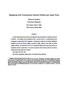
It can be shown (see the Appendix) that the sequence zn is decreasing and converges to 1: For example, for = 2; zn decreases like this: Since zn ! 1; we have that limn!1

re-scaling the problem to disappear too.

3.2

c0 ;1 c

cn cn+1 c

= limn!1

cn cn+1 cn cn c

= 0: After

; it implies that as the gap disappears, the atoms

Dynamics of the Atomless Limit

Since we have shown that the limit of DL equilibria (as the gap disappears) is atomless, we have that in the limit the seller makes zero pro…t (recall that in the DL limit the seller makes money only on the …rst atom). 12

3

zn 2

1

0

10

5

Figure 1:

cn+1 cn

15

20

25

30

in the uniform case for v = 2c:

Also, since we have shown that lim

"!0;n!1

yn (") =

pn (") "!0;n!1 cn (") lim

c =1 c

we get that in the limit P (k) = k In words, given the seller beliefs remaining types are distributed on a range [c; k] ; he asks price k: Since there are no atoms in the limit, that price is accepted by type k only, hence each type pays a price equal to the cost of serving that type. In the gap case the prices are quite complicated and depend on the details of the distribution. As the gap disappears, prices become very simple and independent of the distribution! To …nish describing the limit we only need to pin down K (t) : It is described by a di¤erential equation that guarantees that no type of the buyer wants to postpone or speed up trade: r (v (c)

@pt @t for c = K (t) c) =

13

where pt = P (K (t)) is the equilibrium path of prices over time. This indi¤erence condition can be written as: r (v (K (t))

K (t)) =

K_ (t)

and with a boundary condition K (0) = c (since there is no atom at time 0); it uniquely de…nes K (t) : For example, when v (c) = c for some > 1; c = 0 (so that v (c) = c)) and we normalize c = 1 then we get: K (t) = e

4

r(

1)t

= pt

Durable Goods and the Coase Conjecture.

We can interpret the model also as a durable good problem in the following way. Let v be distributed according to G (v) (which can be obtained from v (c) and the distribution F (c)) and let c (v) v 1 (v) : Then 1 G (v) is the demand function where the total mass of customers has been normalized to 1. Let V (Q) be the corresponding inverse demand function. Let qt be the quantity sold at time t; and Qt be the cumulative sales including time t : Qt = Qt

1

+ qt

Q0 = q0 Assume the following industry-wide experience e¤ects: if the industry sold Qt 1 units by time t and sells qt units at time t then the cost per unit of production at time t is Z

Qt

c (V (q)) dq if qt > 0 qt Qt 1 C (Qt ) = c (V (Qt )) if qt = 0 C (Qt ) =

14

For example, if demand is linear, V (Q) = 1 the bargaining problem is c (v) = v for some C (Qt 1 ; qt ) =

1

1

Q; and the underlying function from > 1; then Qt

1

qt 2

Our assumption that v 0 (c) > 0 implies that the costs of serving customers fall with the cumulative sales. C (Qt ) here corresponds in the bargaining model to the average cost of serving the buyer conditional on a sale, completing the usual analogy between the durable goods and bargaining problems. A competitive equilibrium in this model is described by a sequence of prices 1 fpt g1 t=0 and quantities fqt gt=0 such that: pt = C (Qt ) if qt > 0 pt V (Qt )

C (Qt ) if qt = 0

pt =

(V (Qt )

pt+1 )

The …rst condition is that if there are any sales in period t …rms make zero pro…t. The second condition means that …rms are always willing to supply the product at the current marginal cost, so for sales to be zero it must be that prices are below current marginal costs. The last condition captures buyer optimality: given the sequence of prices buyers choose optimally when to buy. Note that even if the DL equilibrium has zero pro…t in the limit (which is a nongeneric case), it does not satisfy the conditions of competitive equilibrium: during the quiet periods prices are necessarily higher than C (Qt ) : Finally, we stress the positive externality in this market: a …rm producing more today reduces the marginal cost to other …rms both in the current period and in the future. Since a …rm does not capture that increase of total surplus, the competitive equilibrium outcome is ine¢ cient: Qt is growing too slowly. It is e¢ cient to produce immediately at the level where c(Q) = V (Q) ; but the competitive equilibrium is only slowly converging to that total output. In the continuous-time limit prices change continuously over time with pt = C (Qt ) and cumulative sales follow the following 15

process: Q0 = 0 r (V (Qt )

C (Qt )) =

C 0 (Qt ) Q_ t | {z } = p_ t

That implies:5

Proposition 2 (Weak Coase Conjecture) Consider a durable good problem. In the "no gap" case with experience e¤ects, there exists a stationary equilibrium of the monopolist problem that as ! 0 converges to the competitive equilibrium outcome. To reiterate, the Coase Conjecture is not about e¢ ciency of the outcome (as it is often interpreted) but about the monopolist acting in the limit as a competitive industry would. With no experience e¤ects, the competitive equilibrium is e¢ cient, but here it is not. This is consistent with the original Coase (1972) claim that the monopolist without commitment would act no di¤erent than competitive sellers.6 Finally, we call it the "Weak" Coase Conjecture, since we are not able to prove that all stationary equilibria of the monopolist problem converge to the competitive equilibrium outcome (the methods in Fuchs and Skrzypacz (2009) can be used to establish that all stationary equilibria with atomless limit converge, but it is an open question if there could be equilibria of the monopoly problem with atoms of trade in the limit). It is an open question whether a "Strong" version of the conjecture is true (i.e. if all stationary equilibria of the monopolist problem converge to the competitive outcome as ! 0):7 5

This claim was …rst informally discussed in Fuchs and Skrzypacz (2009). Since in the standard model competitive equilibrium is e¢ cient, the Coase conjecture is sometimes interpreted as a claim that the monopolist with commitment will also achieve e¢ ciency. Yet, Coase (1972) stresses the comparison between the competitive and monopolistic markets. 7 Even if all stationary equilibria satisfy the Coase conjecture in the no-gap case there can also also be non-stationary equilibira that violate the Coase Conjecture. See Ausubel and Deneckere (1989) for the construction of such equilibria for the constant marginal cost case. 6

16

5

Appendix

Claim: zn de…ned in equation (9) is decreasing and converging to 1 Proof: Let (z) be: (z) = (2 so that zn+1 =

1)

4( 1)2 (2 1) z1

(zn ) : We have 0

0

2(

1) (z) = (2 1) z 1 0 (1) = 1; (1) = 1; (z) < 1;

2

>0

(z) > z for all z > 1:

That implies that if z0 > 1 then zn > 1 for all n: Also, since (z) < z for all z > 1; we get that the sequence zn is decreasing. Finally, …x any any z > 1: For all z z ; z f (z) is uniformly bounded away from 0 (to see this, note that 0 (z) is uniformly bounded away from 1 for all z z ): That implies that from any zk z there exists a …nite l such that zk+l < z : Therefore, the decreasing (and bounded, hence converging) sequence zn converges to 1:

References [1] Ausubel, Lawrence M., and Raymond J. Deneckere. 1989. “Reputation in Bargaining and Durable Goods Monopoly.”Econometrica, 57(3): 511-531. [2] Bulow Jeremy. 1982 “Durable Goods Monopolists." Journal of Political Economy 90, no. 2, (April 1982):314-32. [3] Coase, Ronald H. 1972. “Durability and Monopoly.” Journal of Law and Economics, 15 (1): 143-149.

17

[4] DeMarzo, Peter M. and Branko Urosevic. 2006. “Ownership Dynamics and Asset Pricing with a Large Shareholder.” Journal of Political Economy, 114(4): 774-815. [5] Deneckere, Raymond J., and Meng-Yu Liang. 2006. “Bargaining with Interdependent Values.”Econometrica, 74(5): 1309-1364. [6] Evans, Robert. 1989. “Sequential Bargaining with Correlated Values.”Review of Economic Studies, 56(4): 499-510. [7] Fuchs, William and Andrzej Skrzypacz. 2009 “Bargaining with Arrival of New Traders.” [8] Fudenberg, Drew, David Levine, and Jean Tirole. 1985. “In…nite-horizon models of bargaining with one-sided incomplete information.” In Game Theoretic Models of Bargaining, ed. Alvin E. Roth, 73-98. Cambridge, MA: Cambridge University Press. [9] Gul, Faruk, Hugo Sonnenschein, and Robert Wilson. 1986. “Foundations of dynamic monopoly and the Coase Conjecture.”Journal of Economic Theory, 39(1): 155-190. [10] Stokey, Nancy L. 1981. “Rational Expectations and Durable Goods Pricing.” Bell Journal of Economics, 12(1): 112-128. [11] Vincent, Daniel R. 1989. “Bargaining with Common Values.”Journal of Economic Theory, 48(1): 47-62.

18