Automaticity, almost convexity and falsification by fellow traveler properties of some finitely generated groups Murray James Elder Submitted in total fulfillment of the requirements of the Degree of Doctor of Philosophy June 2000. Revised September 2000 Department of Mathematics and Statistics The University of Melbourne

Figure 1: Two Openings in Black over Wine, Mark Rothko 1958. The Tate Gallery, London. i

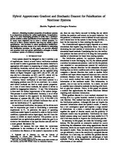
Abstract We set out to examine the automaticity and almost convexity of an intriguing class of groups. Brady and Bridson provide examples from this class with quadratic isoperimetric function that are not biautomatic. Thus showing these examples are automatic would answer a long-standing question in automatic group theory. Wise gives another example from this class which is non-Hopfian and CAT(0). Determining the automaticity of this example would answer one of two questions; are all CAT(0) groups automatic, and are all automatic groups Hopfian? Determining its almost convexity would give similar insight. We start by trying to understand the geodesic structure of the Cayley graphs of these examples, for a particular choice of generating set. This leads us to define the notion of a pattern in the Cayley graph, and we succeed in characterising the set of all patterns for these groups. From this we can prove they are almost convex for the chosen generating sets. This gives the first example of a non-Hopfian almost convex group. We also prove that the full language of geodesics is not regular, and moreover there is no geodesic automatic language for these examples with respect to the chosen generating sets. Neumann and Shapiro define the falsification by fellow traveler property and show that if a group enjoys this property then its full language of geodesics is regular. Consequently the above examples do not enjoy this property. Related to it is the loop falsification by fellow traveler property which we introduce in this thesis. Figure 2 summarises some facts about these properties. The two non-implications shown result from this thesis. We ask whether all groups with a quadratic isoperimetric function enjoy the loop falsification by fellow traveler property. If so we would have a surprising characterisation for these groups. An example of Stallings appears to provide some clues to this question. We also examine the question of higher dimensional finiteness and higher dimensional isoperimetric functions for groups enjoying these geometric properties. We prove that if a group enjoys the falsification by fellow traveler property then it is of type F3 . We ask whether the larger class of almost convex groups are of type F3 . Stallings’ group would be a potential counterexample to this, since it is finitely presented and not of type F 3 . We prove that for two independently arising generating sets, Stallings’ group is

ii

full language of geodesics is regular

?

falsification by fellow traveller property

loop falsification by fellow traveller property

finitely presented

almost convex

?

asynchronous loop falsification by fellow traveller property

at most exponential isoperimetric function

finitely presented

?

at most quadratic isoperimetric function

Figure 2: Implication diagram not almost convex, suggesting it is not almost convex for any generating set.

iii

This is to certify that (i) the thesis comprises only my original work, (ii) due acknowledgment has been made in the text to all other material used, (iii) the thesis is less than 100,000 words in length.

iv

Acknowledgments My thanks to Walter Neumann for his encouragement, ideas and advice, and thanks to Mike Shapiro and to Andrew Rechnitzer for their help throughout my PhD. Thanks to Dean Chequer, Mum and Dad, Alisoun, Bill, Kathy, Esther, Lisa, Megan, Jessica, Suzanne Buchta, Lois Bedson, Janie Burrows, Bell Foozwell, Paul Gregg, Averil Newman, Amanda Johnson and Kerry Williams for their love, patience and support, and thanks to Noel Brady, Martin Bridson and Sarah Rees for their invaluable suggestions.

v

Contents 1 Introduction and Definitions 1.1 Some Open(ing) Questions . . . . . . . . . . . . . . . . . 1.2 Geometric Group Theory . . . . . . . . . . . . . . . . . . 1.3 Almost convex groups . . . . . . . . . . . . . . . . . . . . 1.4 Isoperimetric functions . . . . . . . . . . . . . . . . . . . . 1.5 Regular languages . . . . . . . . . . . . . . . . . . . . . . 1.6 Fellow traveler properties . . . . . . . . . . . . . . . . . . 1.7 Automatic groups . . . . . . . . . . . . . . . . . . . . . . 1.8 Changing weighted generating sets preserves automaticity 1.9 Some other miscellaneous geometric group theory . . . . . 1.9.1 Eilenberg MacLane spaces . . . . . . . . . . . . . . 1.9.2 CAT(0) groups . . . . . . . . . . . . . . . . . . . . 1.9.3 HNN extensions . . . . . . . . . . . . . . . . . . . 1.9.4 Hopficity . . . . . . . . . . . . . . . . . . . . . . . 2 Automaticity and almost convexity for an example of and Bridson 2.1 Introduction . . . . . . . . . . . . . . . . . . . . . . . . 2.2 Asynchronous automaticity . . . . . . . . . . . . . . . 2.3 Geodesic structure and Patterns . . . . . . . . . . . . 2.3.1 Geodesics and “Pre-sequences” . . . . . . . . . 2.3.2 Sequences and Patterns . . . . . . . . . . . . . 2.3.3 An imaginary finite state automaton . . . . . . 2.3.4 Moves . . . . . . . . . . . . . . . . . . . . . . . 2.3.5 Moves as rewriting rules. . . . . . . . . . . . . 2.3.6 Proof of the Conjecture . . . . . . . . . . . . . 2.4 Almost convexity . . . . . . . . . . . . . . . . . . . . . 2.5 Geodesic automatic languages . . . . . . . . . . . . . .

vi

. . . . . . . . . . . . .

1 . 1 . 4 . 8 . 12 . 14 . 15 . 18 . 32 . 35 . 35 . 36 . 36 . 38

Brady . . . . . . . . . . .

. . . . . . . . . . .

. . . . . . . . . . .

. . . . . . . . . . .

39 39 41 46 47 50 52 53 60 63 65 80

3 The 3.1 3.2 3.3 3.4 3.5 3.6 3.7

Wise Group Introduction . . . . . . . . . . . . Asynchronous automaticity . . . Geodesic structure and Patterns Geodesic automatic structures . . Proof of the Conjecture . . . . . Almost convexity . . . . . . . . . Conclusion . . . . . . . . . . . .

. . . . . . .

. . . . . . .

. . . . . . .

. . . . . . .

. . . . . . .

. . . . . . .

. . . . . . .

. . . . . . .

. . . . . . .

. . . . . . .

. . . . . . .

. . . . . . .

. . . . . . .

. . . . . . .

. . . . . . .

. . . . . . .

85 85 86 90 103 107 118 134

4 Finiteness properties, isoperimetric functions, the falsification by fellow traveler property and almost convexity 135 4.1 Introduction . . . . . . . . . . . . . . . . . . . . . . . . . . . . 135 4.2 Finiteness for asynchronously automatic groups . . . . . . . . 136 4.3 Groups with the falsification by fellow traveler property are of type F3 . . . . . . . . . . . . . . . . . . . . . . . . . . . . . 138 4.4 Almost convexity and Stallings’ example . . . . . . . . . . . . 148 4.4.1 Baumslag et al’s presentation . . . . . . . . . . . . . . 148 4.4.2 Bestvina and Brady’s presentation . . . . . . . . . . . 152 4.4.3 Bridson’s presentation . . . . . . . . . . . . . . . . . . 154 4.5 The loop falsification by fellow traveler property and quadratic isoperimetric functions . . . . . . . . . . . . . . . . . . . . . . 155

vii

List of Figures 1 2

Two Openings in Black over Wine, Mark Rothko 1958. The Tate Gallery, London. . . . . . . . . . . . . . . . . . . . . . . Implication diagram . . . . . . . . . . . . . . . . . . . . . . .

i iii

1.1 1.2 1.3 1.4 1.5 1.6 1.7 1.8 1.9 1.10 1.11 1.12 1.13 1.14 1.15 1.16 1.17 1.18 1.19 1.20 1.21 1.22

Γ{a,b} (F2 ) . . . . . . . . . . . . . . . . . . . . . . ΓX (F2 ) . . . . . . . . . . . . . . . . . . . . . . . Making the graph ΓX 0 (G) . . . . . . . . . . . . . γ of length k + m . . . . . . . . . . . . . . . . . . Length at most C(k)2 . . . . . . . . . . . . . . . Growth of the metric ball in a non-almost convex Step 1 . . . . . . . . . . . . . . . . . . . . . . . . Step 2 . . . . . . . . . . . . . . . . . . . . . . . . The Pumping Lemma . . . . . . . . . . . . . . . The falsification by fellow traveler property . . . Geodesics asynchronously k-fellow traveling . . . Case 1.1 . . . . . . . . . . . . . . . . . . . . . . . Case 1.2 . . . . . . . . . . . . . . . . . . . . . . . Case 1.3 . . . . . . . . . . . . . . . . . . . . . . . Case 2.1 . . . . . . . . . . . . . . . . . . . . . . . Case 2.2 . . . . . . . . . . . . . . . . . . . . . . . Case 3.1 . . . . . . . . . . . . . . . . . . . . . . . Case 3.2 . . . . . . . . . . . . . . . . . . . . . . . Case 4 . . . . . . . . . . . . . . . . . . . . . . . . Showing LY has the fellow traveler property . . . Padding the words so that they fellow travel . . . Cyclic subgroups of 2 . . . . . . . . . . . . . . .

5 5 6 9 10 10 11 11 15 16 17 22 24 24 25 27 28 29 30 34 35 37

2.1 2.2

π1 (S 1 ) = = hai, B2,3 = ha, t | t−1 a2 t = a3 i . . . . . . . . . . 40 π1 (T ) = 2 = ha, b | ab = bai. We choose cyclic subgroups hai, habi and hab−1 i. . . . . . . . . . . . . . . . . . . . . . . . 40

viii

. . . . . . . . . . . . . . . . . . . . group . . . . . . . . . . . . . . . . . . . . . . . . . . . . . . . . . . . . . . . . . . . . . . . . . . . . . . . . . . . . . . . .

. . . . . . . . . . . . . . . . . . . . . .

. . . . . . . . . . . . . . . . . . . . . .

. . . . . . . . . . . . . . . . . . . . . .

2.3 2.4 2.5 2.6 2.7 2.8 2.9 2.10 2.11 2.12 2.13 2.14 2.15 2.16 2.17 2.18 2.19 2.20 2.21 2.22 2.23 2.24 2.25 2.26 2.27 2.28 2.29 2.30 2.31 2.32 2.33 2.34 2.35 2.36 2.37 2.38 2.39 2.40 2.41

A presentation 2-complex for ha, b, s, t | ab = ba, s −1 as = ab, t−1 at = ab−1 i. . . . . . . . . . . . . . . . . . . . . . . . . . A 2-combing of 2 . . . . . . . . . . . . . . . . . . . . . . . . rn = s−1 , x = ab . . . . . . . . . . . . . . . . . . . . . . . . . rn = s, x = b . . . . . . . . . . . . . . . . . . . . . . . . . . . rn = s, x = ab−1 . . . . . . . . . . . . . . . . . . . . . . . . . A 2 plane . . . . . . . . . . . . . . . . . . . . . . . . . . . . An s-strip . . . . . . . . . . . . . . . . . . . . . . . . . . . . . Coset representatives for a normal form language . . . . . . . w0 = c2 b, r1 = s−1 . . . . . . . . . . . . . . . . . . . . . . . . (All) geodesics to the first strip. . . . . . . . . . . . . . . . . . The next plane for w = c2 s−1 d−2 bs−1 . . . . . . . . . . . . . . Determining the next pre-sequence for w. . . . . . . . . . . . Exiting the second plane by a different strip. . . . . . . . . . “Initial patterns” (−1)(0)(1) . . . . . . . . . . . . . . . . . . “Parallel moves” . . . . . . . . . . . . . . . . . . . . . . . . . Move 2 gives (−1)(0)(10)(1) . . . . . . . . . . . . . . . . . . . Another move 2 gives (−1)(0)(10)(1110)(1) . . . . . . . . . . Another move 2 gives (−1)(0)(10)(1110)(1 7 0)(1) . . . . . . . A potentially “bad” pattern . . . . . . . . . . . . . . . . . . . Move 1 . . . . . . . . . . . . . . . . . . . . . . . . . . . . . . . Move 2: c/d → a . . . . . . . . . . . . . . . . . . . . . . . . . Move 3: a → c/d . . . . . . . . . . . . . . . . . . . . . . . . . Move 4: c/d → d/c . . . . . . . . . . . . . . . . . . . . . . . . γ = r 1 r2 . . . . . . . . . . . . . . . . . . . . . . . . . . . . . . γ = rx . . . . . . . . . . . . . . . . . . . . . . . . . . . . . . . Last strip is s, t . . . . . . . . . . . . . . . . . . . . . . . . . . γ1 . . . . . . . . . . . . . . . . . . . . . . . . . . . . . . . . . γ2 . . . . . . . . . . . . . . . . . . . . . . . . . . . . . . . . . γ3 . . . . . . . . . . . . . . . . . . . . . . . . . . . . . . . . . γ4 . . . . . . . . . . . . . . . . . . . . . . . . . . . . . . . . . γ5 . . . . . . . . . . . . . . . . . . . . . . . . . . . . . . . . . γ6 . . . . . . . . . . . . . . . . . . . . . . . . . . . . . . . . . γ7 . . . . . . . . . . . . . . . . . . . . . . . . . . . . . . . . . γ8 . . . . . . . . . . . . . . . . . . . . . . . . . . . . . . . . . Last strip is s−1 , t−1 . . . . . . . . . . . . . . . . . . . . . . . γ1 . . . . . . . . . . . . . . . . . . . . . . . . . . . . . . . . . γ2 . . . . . . . . . . . . . . . . . . . . . . . . . . . . . . . . . γ3 . . . . . . . . . . . . . . . . . . . . . . . . . . . . . . . . . γ4 . . . . . . . . . . . . . . . . . . . . . . . . . . . . . . . . . ix

41 42 43 43 44 45 45 47 48 48 49 50 51 54 55 56 57 58 59 60 61 62 63 66 67 67 68 68 69 69 70 71 71 72 72 73 74 74 75

2.42 2.43 2.44 2.45 2.46 2.47 2.48 2.49 2.50 2.51 2.52

γ5 . . . . . . . . . . . . . . . . . . . . . . . . . . . . . . γ6 . . . . . . . . . . . . . . . . . . . . . . . . . . . . . . γ7 . . . . . . . . . . . . . . . . . . . . . . . . . . . . . . γ8 . . . . . . . . . . . . . . . . . . . . . . . . . . . . . . Finding a sequence of the form (−1)1000(1) . . . . . . . The lower bound for the almost convexity constant is 6 Finding a sequence 1k 0 . . . . . . . . . . . . . . . . . . . A parallel move to get on a different branch . . . . . . . “Undoing” the pattern . . . . . . . . . . . . . . . . . . . Unique geodesics that don’t fellow travel . . . . . . . . . The language of geodesics for G 1,1 ,Y is not regular . . .

. . . . . . . . . . .

76 76 77 78 79 79 80 81 82 83 84

3.1 3.2 3.3 3.4 3.5 3.6 3.7 3.8 3.9 3.10 3.11 3.12 3.13 3.14 3.15

A Euclidean 2-complex which satisfies the link condition. . . A 1-combing for 2. . . . . . . . . . . . . . . . . . . . . . . . rn = s−1 , x = b . . . . . . . . . . . . . . . . . . . . . . . . . . rn = s, x = b−1 . . . . . . . . . . . . . . . . . . . . . . . . . . Initial sequences (a/b). . . . . . . . . . . . . . . . . . . . . . . Initial sequences (c). . . . . . . . . . . . . . . . . . . . . . . . c→c. . . . . . . . . . . . . . . . . . . . . . . . . . . . . . . . c → c again. . . . . . . . . . . . . . . . . . . . . . . . . . . . . a/b → a/b . . . . . . . . . . . . . . . . . . . . . . . . . . . . . c → a/b . . . . . . . . . . . . . . . . . . . . . . . . . . . . . . c → a/b again. . . . . . . . . . . . . . . . . . . . . . . . . . . c → c Parallel move. . . . . . . . . . . . . . . . . . . . . . . . a/b → a/b Parallel move. . . . . . . . . . . . . . . . . . . . . Move 3: a/b → c . . . . . . . . . . . . . . . . . . . . . . . . . Move 4: a/b → b/a. The pattern here is not of conjectured form, hence the bad pattern produced. . . . . . . . . . . . . gak is geodesic but gak+1 is not. . . . . . . . . . . . . . . . . (G, X) has the loop falsification by fellow traveler property . Two unique geodesics that don’t fellow travel. . . . . . . . . . γ is half the edge r. . . . . . . . . . . . . . . . . . . . . . . . . γ is half the edge r1 and half the edge r2 . . . . . . . . . . . . γ is half an edge r and half an a or b. . . . . . . . . . . . . . γ is half an edge r and half a c. . . . . . . . . . . . . . . . . . Possibilities for γ when last strip is an s or t. . . . . . . . . . γ1 . . . . . . . . . . . . . . . . . . . . . . . . . . . . . . . . . . γ2 . . . . . . . . . . . . . . . . . . . . . . . . . . . . . . . . . . γ3 . . . . . . . . . . . . . . . . . . . . . . . . . . . . . . . . . . γ4 . . . . . . . . . . . . . . . . . . . . . . . . . . . . . . . . . .

86 87 88 88 90 91 92 93 94 95 96 98 99 100

3.16 3.17 3.18 3.19 3.20 3.21 3.22 3.23 3.24 3.25 3.26 3.27

x

. . . . . . . . . . .

. . . . . . . . . . .

102 104 104 106 119 120 120 121 122 122 123 123 123

3.28 3.29 3.30 3.31 3.32 3.33 3.34 3.35 3.36 3.37 3.38 3.39 3.40 3.41 3.42 3.43 3.44 3.45 3.46 3.47 3.48 3.49

γ5 . . . . . . . . . . . . . . . . γ6 . . . . . . . . . . . . . . . . γ7 . . . . . . . . . . . . . . . . γ8 . . . . . . . . . . . . . . . . γ9 . . . . . . . . . . . . . . . . Possible paths for γ when last γ1 . . . . . . . . . . . . . . . . γ2 . . . . . . . . . . . . . . . . γ3 . . . . . . . . . . . . . . . . γ4 . . . . . . . . . . . . . . . . γ5 . . . . . . . . . . . . . . . . γ6 . . . . . . . . . . . . . . . . γ7 . . . . . . . . . . . . . . . . γ8 . . . . . . . . . . . . . . . . γ9 . . . . . . . . . . . . . . . . γ10 . . . . . . . . . . . . . . . . γ11 . . . . . . . . . . . . . . . . γ12 . . . . . . . . . . . . . . . . The path to ∗ has no c’s. . . γ13 . . . . . . . . . . . . . . . . γ14 . . . . . . . . . . . . . . . . Proving C(1) ≥ 4. . . . . . .

4.1

The falsification by fellow traveler property implies almost convexity. . . . . . . . . . . . . . . . . . . . . . . . . . . . . . φ(i + 1) < j + 1 . . . . . . . . . . . . . . . . . . . . . . . . . . φ(i + 1) ≥ j + 1 . . . . . . . . . . . . . . . . . . . . . . . . . . The drum construction . . . . . . . . . . . . . . . . . . . . . . A side cell . . . . . . . . . . . . . . . . . . . . . . . . . . . . . The “tear” in the base . . . . . . . . . . . . . . . . . . . . . . Base type 1 . . . . . . . . . . . . . . . . . . . . . . . . . . . . Base type 2 . . . . . . . . . . . . . . . . . . . . . . . . . . . . Paths in ΓX (S). . . . . . . . . . . . . . . . . . . . . . . . . . . Changing the path P keeping the edge s −1 fixed. . . . . . . . σc,d ≡ v −1 . . . . . . . . . . . . . . . . . . . . . . . . . . . . The octahedron ∆ . . . . . . . . . . . . . . . . . . . . . . . . Paths in ΓY (S) . . . . . . . . . . . . . . . . . . . . . . . . . . A geodesic g to αu . . . . . . . . . . . . . . . . . . . . . . . . A potential counterexample to the loop falsification by fellow traveler property for S, Y. . . . . . . . . . . . . . . . . . . . .

4.2 4.3 4.4 4.5 4.6 4.7 4.8 4.9 4.10 4.11 4.12 4.13 4.14 4.15

xi

. . . . . . . . . . . . . . . strip . . . . . . . . . . . . . . . . . . . . . . . . . . . . . . . . . . . . . . . . . . . . . . . .

. . . . . . . . . . . . . . . . . . . . . . . . . . . . . . . . . . . is s −1 , t−1 . . . . . . . . . . . . . . . . . . . . . . . . . . . . . . . . . . . . . . . . . . . . . . . . . . . . . . . . . . . . . . . . . . . . . . . . . . . . . . . . . . . . . . . . . . . . . . . . . . . . . . . . . . . . . . . . .

. . . . . . . . . . . . . . . . . . . . . .

. . . . . . . . . . . . . . . . . . . . . .

. . . . . . . . . . . . . . . . . . . . . .

. . . . . . . . . . . . . . . . . . . . . .

. . . . . . . . . . . . . . . . . . . . . .

. . . . . . . . . . . . . . . . . . . . . .

. . . . . . . . . . . . . . . . . . . . . .

. . . . . . . . . . . . . . . . . . . . . .

124 124 125 125 126 126 126 127 127 128 128 129 129 129 130 130 131 131 132 132 133 133 138 140 140 142 143 144 145 146 149 150 151 152 154 155 157

4.16 A potential counterexample to the loop falsification by fellow traveler property for S, X . . . . . . . . . . . . . . . . . . . . . 158 4.17 An even worse loop in S, X . . . . . . . . . . . . . . . . . . . . 159

xii

Chapter 1

Introduction and Definitions 1.1

Some Open(ing) Questions

This thesis sets out to examine some important geometric and machinetheoretic properties of groups. We start by defining these properties, and then consider some carefully chosen examples of groups for which the enjoyment of the properties would have some important consequences. We are motivated by the following open questions, which we will discuss presently before defining terms below. The first question is fundamental in the theory of automatic groups. An automatic structure for a group is a set of words in the letters of some generating set for the group, called a language, so that this language is regular and satisfies a fellow traveler property. We will discuss these ideas more thoroughly below. We say a group is automatic if it admits some automatic structure. A group is biautomatic if it has an automatic structure such that the inverse of the language (that is, all words read backwards) is also automatic. Clearly biautomatic groups are automatic. Open Question 1. Does every automatic group admit some biautomatic structure? This question is probably as old as the theory of automatic groups itself, which is not all that old. It is certainly not true that every automatic structure for a group is biautomatic, for example [ECHLPT] Example 4.4.1 has an automatic structure whose inverse is not automatic. One useful invariant for a finitely presented group is the geometrically motivated isoperimetric function. Various classes of groups have certain bounds on the type of isoperimetric functions allowed; Automatic groups have at most quadratic isoperimetric functions ([ECHLPT] Theorem 2.3.12). 1

Brady and Bridson [BrBr2] have recently determined a class of groups that are not biautomatic and have quadratic isoperimetric function, so these groups are good candidates for a counterexample. In Chapter 2 we consider one of these groups and try to find a synchronous automatic structure. Euclidean groups and hyperbolic groups in the sense of Gromov are easily shown to be automatic. So we might expect to find automatic structures for CAT(0) groups as easily. Niblo and Reeves [NR1] prove that groups which act on CAT(0) cube complexes admit a biautomatic structure. This extends a result of Gersten and Short [GS2] which shows that groups which act on CAT(0) 2-complexes constructed from Euclidean squares or equilateral triangles are automatic. Open Question 2. Is every CAT(0) group automatic? Wise [W1] considered a now infamous example of a (non-Hopfian) CAT(0) group that seemed a likely candidate for an automatic structure. In Chapter 3 we study this example in detail, and work hard to find a synchronously automatic structure, without success. A group is Hopfian if every epimorphism from the group to itself is an isomorphism. The class of Hopfian groups is of considerable interest. If Wise’s example is in fact automatic we could resolve the following. Open Question 3. Is every automatic group Hopfian? A geometric property that is closely related to automaticity is that of almost convexity. Cannon defines the concept in [C1] where he gives a simple and efficient solution to the word problem for almost convex groups. The property of almost convexity is generating set dependent, as was shown by Theil [T], so is not a group invariant. Shapiro and Stein [SS] show that the fundamental groups of closed 3-manifolds carrying one of Thurston’s eight geometries except solvgeometry are almost convex, following Cannon et al [CFGT] who prove that no co-compact discrete group based on solvgeometry is almost convex. Hyperbolic groups and Euclidean groups are almost convex [C1]. So intuitively groups admitting non-positively curved geometry of some kind are almost convex. This suggests the following. Open Question 4. Are all CAT(0) groups almost convex? We might also ask: Open Question 5. Are all almost convex groups Hopfian?

2

The example of Wise is CAT(0) and non-Hopfian, and we will show that for at least one choice of generating set this group is almost convex. Thus we supply an answer to this previously open question. We also consider the falsification by fellow traveler property, introduced by Neumann and Shapiro in [NS3] and credited to Cannon, which is closely related to almost convexity and automaticity. It is easily shown that groups that enjoy the falsification by fellow traveler property are almost convex, and we give a proof of this in Chapter 4. Neumann and Shapiro prove that groups that enjoy the falsification by fellow traveler property have a regular language of geodesics [NS3]. They also show it is a generating set dependent property. We then ask how the above properties of groups determine the finiteness of groups, in particular the finiteness property F n , introduced by Wall [Wa]. Bieri later introduced a related homological finiteness property FP n and both are discussed frequently in the literature. F n implies FPn and it was a long-standing question if the converse holds. Bestvina and Brady give a good overview of these properties in [BeBr], and in particular resolve this question negatively. Alonso [A1] proves that groups with a “bounded combing” are of type FPn for any n ∈ ; Gersten proves that asynchronously combable groups with departure function are of type F 3 in [CDS], and indicates that the proof of Fn for any n is similar. It follows that asynchronously automatic groups are of type Fn for all n. In Chapter 4 we adapt Gersten’s proof to groups that enjoy the falsification by fellow traveler property and succeed in showing such groups are of type F3 . The proof involves considerably more subtlety, and does not appear to generalize, so two remaining open questions are: Open Question 6. For which natural numbers n are groups that enjoy the falsification by fellow traveler property of type F n ? Open Question 7. For which natural numbers n are almost convex groups of type Fn ? Almost convex groups are finitely presented so we know they are of type F2 . In the final sections we discuss another example that could potentially answer this question, namely a group first given by Stallings [St1] that is finitely presented but not of type FP 3 hence not F3 . We introduce a modified version of the falsification by fellow traveler property restricted to loops, called the loop falsification by fellow traveler property, and show that if a group enjoys this property then it has at most quadratic isoperimetric function. If the converse were true we would have an interesting geometric 3

characterization for the menagerie of groups having quadratic isoperimetric functions (Gersten calls them a “zoo” in [G1]). Open Question 8. If G has a quadratic isoperimetric function then does G enjoy the loop falsification by fellow traveler property? Bridson [B] has recently shown Stallings’ group has exactly a quadratic isoperimetric function. Surprisingly we find that for the given generating sets, Stallings’ group does not appear to enjoy the loop falsification by fellow traveler property. So it is likely this last question can be answered negatively. We have included these open questions at the outset to serve as motivation for the choices of the examples we will consider below. For the remainder of this chapter we will give precise definitions and work through the basic consequences of the properties we are to consider.

1.2

Geometric Group Theory

Geometric Group Theory is the study of groups from a geometric point of view. Every group with a given generating set gives rise to a Cayley graph, and we define the more general notion of a weighted Cayley graph as follows. Definition 1.1. Suppose G is a group with weighted generating set X. That is, for each x ∈ X we have a rational weighting ω x > 0. Suppose further that X is inverse closed, and that ωx = ωx−1 . The weighted Cayley graph ΓX (G) for G with respect to X is the directed graph with vertices labeled g for each g ∈ G, and directed edges labeled x from g to g 0 of length ωx whenever g 0 = gx for some x ∈ X. It is worth considering an easy example at this point, to see how beautiful and revealing this construction is. Take the group F 2 ∼ = ha, b | −i which is the free group on two generators, a pretty straightforward infinite group. The Cayley graph Γ{a,b} (F2 ) is shown in Figure 1.1. Suppose we took a weighted generating set X = {a, b : wa = 1, wb = 2}. Then the Cayley graph with respect to this generating set is shown in Figure 1.2. The reader unfamiliar with this construction is encouraged to look at [ECHLPT] pages 34-39. Changing the relative weightings of generators changes the geometry of the Cayley graph. Multiplying all weightings by the same amount simply scales the graph so has no effect on the geometry. If X is a weighted generating set then define the greatest common divisor to be the greatest positive rational number m so that ωx = mx m for some mx ∈ for each x ∈ X. 4

a ab-1

a

ab a

-1

b

ba

b

b-1

b

1

ba -1

a-1

a-1

Figure 1.1: Γ{a,b} (F2 ) a

b

-1

b 1

a -1

Figure 1.2: ΓX (F2 ) Then the set {mx ∈ : x ∈ X} is invariant under scaling. Vertices in the Cayley graph occur at distances in m from the identity. We will make use 5

of a graph ΓX 0 (G) obtained by subdividing each edge x into ω x sub-edges each of length m, as in Figure 1.3. We call the original vertices correspondxi

xi

xi

xi

xi

Figure 1.3: Making the graph ΓX 0 (G) ing to group elements real and the intermediate vertices non-real. We call this graph the subdivided Cayley graph for G, X, and note that it does not correspond to the Cayley graph of any group if m 6= 1. We call the set of edges X 0 = {x01 , . . . , x0n : ωx0i = m ∀xi ∈ X} the subdivided (generating) set corresponding to X. Define the path metric on ΓX (G) by d(g, g 0 ) = min{length of edge path from g to g 0 } for any two vertices g, g 0 , which extends naturally to interior points of edges in the graph. Then we obtain a geodesic metric space, where a geodesic is the shortest edge path between two points. Let X ∗ denote the set of all words in the letters of X ±1 , including the empty word . Any word in X ∗ represents an edge path in the Cayley graph; we shall routinely confuse words and edge paths. We denote the group element represented by a word w ∈ X ∗ by w, and write w =G u if w and u each evaluate to the same group element in G. In terms of the Cayley graph w is the point reached by traversing a path labeled w from the identity. It makes sense therefore to define w for any word w ∈ (X 0 )∗ to be the point in ΓX 0 (G) reached from the identity by the edge path w, whenever such a path exists. The length of a path w ∈ X ∗ is denoted |w| and if g ∈ G is a group element the notation |g| will mean the length of a geodesic for g. A rectifiable path w in a metric space can be parameterized by nonnegative t ∈ by defining w(t) as the point distance t along the path if t < |w| and w(t) = w if t ≥ |w|. We can extend this to all by defining w(t) = w(0) for all t < 0, which will sometimes be convenient. We denote a sub-path of a path w running between points w(i) and w(j) with i ≤ j by [w(i), w(j)]. Let w be a path in the Cayley graph and w(i), w(j) two points along it,

6

for some i ≤ j. The distance d(w(i), w(j)) from w(i) to w(j) in the Cayley graph will be at most the length of the sub-path [w(i), w(j)], which is i − j. We say a path w is quasi-geodesic if there exist constants K > 1,  > 0 such that for all points w(i), w(j) on w, i, j ∈ , 1 |i − j| −  ≤ d(w(i), w(j)) ≤ K|i − j| + . K An isometry is a distance preserving map between metric spaces, that is φ : X → Y is an isometry if φ is surjective and d X (x, x0 ) = dY (φ(x), φ(x0 )) for all points x, x0 ∈ X. A map φ of a metric space X to Y is a quasi-isometry if φ is surjective and there exist constants K,  > 0 such that 1 dX (x, x0 ) −  ≤ dY (φ(x), φ(x0 )) ≤ KdX (x, x0 ) +  K for all points x, x0 ∈ X. G acts by isometries on ΓX (G) by a left action. For all h ∈ G, h : ΓX (G) → ΓX (G) sends vertices g 7→ hg and edges (g, g 0 ) = (g, gx) 7→ (hg, hgx) = (hg, hg 0 ). This action is discrete and co-compact. Now suppose there is a proper geodesic metric space K such that G acts co-compactly and discretely by isometries. Milnor’s Theorem states that K is quasi-isometric to ΓX (G). Put simply, every space on which a group acts in an appropriate way is quasi-isometric to any other. Thus studying the geometry of any such space should provide insight into the geometric properties of the group. ˇ Proofs of this result sometimes attributed to Milnor and/or Svarc can be found in [G1], [Tr]. Note that this result shows that up to quasi-isometry all Cayley graphs for G with respect to any finite generating set are equivalent. A change of weightings of a generating set X induces a quasi-isometry of ΓX (G). (Proposition 11.2.4 [ECHLPT]. Here they say pseudo-isometry.) We can see this clearly in the free group example above. Almost a century ago Max Dehn posed three important questions [D], two of which we will consider here. Suppose you have a group G and a set of generators X for G. Let X ∗ be the set of all words on X. The word problem asks for an algorithm to decide whether any two words u, v on the letters of X are equal in G. Equivalently it asks for an algorithm to decide whether a given word w ∈ X ∗ is equal to the identity in G. The conjugacy problem asks for an algorithm to decide whether two words u, v ∈ X ∗ represent conjugate elements in G. That is, is u =G g −1 vg for some g ∈ G? It is clear that a solution to the conjugacy problem for a given group implies a solution to the word problem for that group. It is also clear that if you have a solution

7

to either problem for one finite generating set, then you can formulate an algorithm for any other finite generating set. It turns out there are groups having insoluble word problem; this amazing result was proved indepently by Boone and Novikov in the 1950’s, and a readable proof is found in [R]. Theorem 1.1. G, X has soluble word problem if and only if there is an algorithm to construct any finite portion of Γ X (G). It is easy to see why this theorem is true: given a word w ∈ X ∗ , if we can construct the portion of the Cayley graph containing w based at the identity vertex, then we can check to see if it is a closed loop; The converse is not much harder.

1.3

Almost convex groups

Cannon [C1] introduced the notion of an almost convex group to understand the efficiency of building the Cayley graph of a group. To motivate the definition consider the task of drawing the Cayley graph of a given group with generating set X. Where would you start? How efficient and logically complicated would your method be? In practice we might start with the identity, and draw all edges out of it. Each edge leads to a new vertex in ΓX . Then from each of these vertices there are edges for each x ∈ X. Of course some take you to vertices you’ve already drawn. If a group is almost convex, then there is an efficient algorithm to construct the metric ball of radius n in ΓX for any n. In practice the algorithm involves a very small list of things to check to decide whether the new edges you draw lead to new vertices or previously drawn ones. The property is a condition on the geometry of the space ΓX . Let G be a group with finite weighted generating set X. Recall the greatest common divisor for X is the greatest positive rational number m such that ωx = mx m for some mx ∈ for each x ∈ X. Define S(n) = {g ∈ ΓX (G) : |g| = n} to be the sphere of radius n and B(n) = {g ∈ ΓX (G) : |g| ≤ n} to be the ball of radius n, for n ∈

≥0 .

8

Definition 1.2. For k ∈ m , G, X is almost convex(k) if there is a constant C(k) > 0 so that for every g, g 0 ∈ S(n), n ∈ m with d(g, g 0 ) ≤ k, there exists a path of length ≤ C(k) inside B(n) from g to g 0 . Proposition 1.1. If G, X is almost convex(k) with k ≥ 2m, then it is almost convex(k + m), and C(k + m) is a function of C(k). Proof: This is proved in [C1] for unweighted generating sets and can be easily modified for the weighted case as follows. Let g, g 0 ∈ S(n), n ∈ m such that d(g, g 0 ) ≤ k + m, realized by γ. If d(g, g 0 ) ≤ k then by hypothesis there is a path of length at most C(k). So assume d(g, g 0 ) = k + m ≥ 3m. If γ ⊆ B(n) then we have a path of length |γ| = k + m. If there is some i ∈ (0, k], i ∈ m such that γ(i) ∈ S(n) then we have a path of length at most 2C(k) from g to γ(i) to g 0 inside B(n). So assume γ has no interior points inside B(n). Thus γ(m), γ(k) ∈ S(n + m), they are distinct since |γ| ≥ 3m, and d(γ(m), γ(k)) = k − m ≤ k. γ(m)

γ γ( k)

g

g

Figure 1.4: γ of length k + m By hypothesis there is a path P of length at most C(k) from γ(m) to γ(k) inside B(n + m). For all i ∈ [0, |P |), i ∈ m one of P (i), P (i + m) ∈ B(n), for if not the edge between them lies outside B(n + m), as shown in Figure 1.5. Therefore one can check that there is a path of length at most C(k) 2 from g to g 0 inside B(n). So putting C(k + m) = max{k + m, 2C(k), C(k) 2 } proves our result. Hence we say G, X is almost convex if it is almost convex(2m). As an illustration of the property, a group is not almost convex if the growth of its ball of radius n looks like Figure 1.6. Hence the “convex” bit. See Cannon [C1] for the following result. Theorem 1.2. If G, X is almost convex, then there exists an algorithm that produces edges and vertices of the Cayley graph Γ X (G) at a constant rate. It follows that the word problem for almost convex groups is solvable. 9

γ n+m n

n+m n

n

n

n n

Figure 1.5: Length at most C(k)2

1

1

1

1

B(0)

Figure 1.6: Growth of the metric ball in a non-almost convex group Proposition 1.2. If G, X is almost convex then G is finitely presented. Proof: Let m be the greatest common divisor of the ω xi . Suppose G is almost convex with respect to the finite generating set X with constant

10

C(2m) = C. We will show that G has presentation hX

| {r =G 1 : |r| ≤ C + 2m}i.

Suppose w =G 1, w ∈ X ∗ . Then w describes a path in ΓX 0 (G) which starts and ends at a real vertex. Let n = min{n 0 ∈ m : w(t) ∈ B(n0 ) ∀t ∈ m }. Then there is some discrete set of points of w that lie in S(n). 1. Let i ∈ m mod |w|. If w(i), w(i + m) ∈ S(n) then by almost convexity there is a path of length at most C from w(i) to w(i + 1) inside B(n), as shown in Figure 1.7. Thus we can replace the sub-path w(i)

w(i+m)

Figure 1.7: Step 1 [w(i), w(i + m)] by this path using a relation of length at most C + m. Adding such a relation for each pair w(i), w(i+m) ∈ S(n), we obtain a new path u such that u =G 1, u ∈ X ∗ and no pair u(i), u(i+m) ∈ S(n). 2. Let i ∈ m mod |u|. If u(i) ∈ S(n) then u(i−m), u(i+m) ∈ S(n−m) By almost convexity there is a path from u(i−m) to u(i+m) of length at most C inside B(n − m), as in Figure 1.8. Thus adding a relation u(i) u(i-m)

u(i+m)

Figure 1.8: Step 2 of length at most C + 2m for each point u(i) ∈ S(n) gives a new path 11

v such that v =G 1, v ∈ X ∗ and v(t) ∈ B(n − m) for all t ∈ m . Then inductively we can fill the loop w by relations of length ≤ C + 2m.

We will use this result in Chapter 4. We see from this proof how Cannon’s results can be modified for weighted generating sets.

1.4

Isoperimetric functions

The previous proposition gives us a way to “fill” any edge loop w = G 1 in a Cayley graph for G, X by relators of bounded size. This suggests a kind of “area” for words w =G 1, w ∈ X ∗ which leads us to a very useful invariant for finitely presented groups called the isoperimetric function. In elementary geometry the isoperimetric problem is concerned with finding the greatest area enclosed by all figures of equal perimeter [We]. If we apply this idea to our geometric group constructions we obtain a useful invariant for finitely presented groups, as well as gaining new insight into their structure. Of course the Cayley graph as defined is a 1-dimensional graph, so we make use of a 2-dimensional Cayley complex defined as follows. Given a group G with presentation hX | Ri construct a 2-complex having one vertex, an edge loop for each generator, and a 2-cell with perimeter labeled by an edge loop for each relator, glued to the 1-skeleton by edge identification. This is sometimes called the presentation 2-complex for G. The Cayley complex is the universal cover of this space. Its 1-skeleton is exactly the Cayley graph for G, X. Epstein et al call it the “filled Cayley graph”. Define the area of a word w =G 1, w ∈ X ∗ to the the minimum number of factors in an expression for w as a product of conjugates of relators in R and their inverses, and denoted as AreaX,R (w). Geometrically the area of w =G 1, w ∈ X ∗ is the minimum number of 2-cells required to fill the edge loop w in the filled Cayley graph for G = hX | Ri. Clearly this definition depends on the choice of presentation. Definition 1.3. The isoperimetric function for G with respect to the presentation hX | Ri is a function δX,R : → defined by δX,R (n) = max{AreaX,R (w) : l(w) ≤ n}. Since there are only a finite number of words w = G 1, w ∈ X ∗ of length at most n, δX,R (n) is a well defined integer.

12

If f, g :→ are two functions from to exist constants A, B, C, D, E > 0 such that

then we say f ≺ g if there

f (n) ≤ Ag(Bn + C) + Dn + E for all n ∈ . We say f is equivalent to g, denoted f ∼ g, if both f ≺ g and g ≺ f . Alonso [A2] proves that if two finite presentations have quasiisometric Cayley graphs then their isoperimetric functions are equivalent, which extends a result of Gersten. So each group has a unique isoperimetric function up to this equivalence. Furthermore it can be checked that if 0 d, d0 ≥ 1 and xd ∼ xd then d = d0 . Thus we say that the isoperimetric function for a given group is polynomial of degree d, exponential, recursive and so on. These results can be read in Gersten [G2] where he proves that a finite presentation has solvable word problem if and only if its isoperimetric function is recursive. Corollary to the proof of Proposition 1.2. If G, X is almost convex then G has at most an exponential isoperimetric function. Proof: Let w =G 1, w ∈ X ∗ such that n = min{n0 ∈ m : w(t) ∈ B(n0 ) ∀t ∈ m } as before. At most |w| applications of step 1 then at most C|w| applications of step 2 gives a word of length at most C 2 |w| with vertices inside B(n − m). This requires the addition of at most |w| + C|w| = c|w| 2-cells for a constant c. By isometry we may assume that w starts at the identity vertex of ΓX (G), so n ≤ 12 |w|. So after 21 |w| iterations we can fill w with 2-cells until it collapses to B(0) which will be the identity vertex. This requires at most 1

2

c|w| + c |w| + . . . + c

1 |w| 2

|w| = |w|

|w|

2 X

ci ≤ |w|d|w| ≤ f |w|

i=1

for constants d, f . An exponential isoperimetric function does not seem like much of a restriction for deciding whether a group is almost convex. We will see below that other classes of groups have much stricter bounds for isoperimetric functions, so this will indeed prove a useful invariant for distinguishing groups in these classes. An intriguing question is to determine the spectrum of all possible exponents for isoperimetric functions. We will see in Chapter 2 that this has been answered by Brady and Bridson [BrBr1]. In Chapter 4 we will introduce a generalization of isoperimetric functions to higher dimensions. 13

1.5

Regular languages

Automatic Group Theory is the study of groups from a machine-theoretic point of view. The idea is to use machines called finite state automata to understand group structure. An alphabet X is any set of letters, and X ∗ is the set of all possible words including the empty word  in letters of X. A (deterministic) finite state automaton M is a machine described by a quintuple (X, S, τ, s0 , A), satisfying the following conditions: 1. M has alphabet X. 2. S is a finite set of states for M 3. τ : S × X → S is the transition function, which tells the machine to which state it must change after reading an element of X 4. s0 ∈ S is the start state 5. A ⊆ S is a set of accept states. M functions by reading words w ∈ X ∗ as follows. M starts in state s0 , reads the first letter of w, and changes to another state as determined by τ . It continues reading letters and changing states until it has read w. If the final state is an accept state we say w is accepted by M . Otherwise w is not accepted. We can also think of M as a graph, with vertex set S, and edges labeled by X determined by τ . That is, there is a directed edge from s 1 to s2 labeled x if τ (s1 , x) = s2 . Now the graph M accepts a word w ∈ X ∗ if after tracing a path from s0 it ends at an accept state. The set of all words in X ∗ accepted by a finite state automaton M is called the language of M and denoted L(M ). If some set of words L ⊂ X ∗ is the language of some finite state automaton then we say L is regular. If w ∈ L we say w is an L-word. M is a non-deterministic finite state automaton if its transition function can take more than one value for any given input. A string is accepted if there is some way to get from the start state to an accept state. A somewhat surprising fact is that if L is accepted by a non-deterministic finite state automaton then L is accepted by a deterministic finite state automaton. If L ⊆ X ∗ is a language let L−1 be the set of all L-words written backwards, and let L∗ be the set of all words including the empty word  in the words of L. 14

Proposition 1.3. If L, L1 , L2 ⊆ X ∗ are regular languages then L−1 , L1 ∪ L2 , L1 ∩ L2 , L∗ are regular languages on X ∗ . The proof can be found in [HU], and is a fun exercise in building nondeterministic automata from the automata for L, L 1 , L2 . A simple yet powerful result about regular languages is the following. Lemma 1.1. (Pumping Lemma) Let M be a finite state automaton on an alphabet X, having n states. If w ∈ L(M ) is a word of length greater than n then we can write w = uzv with |z| > 0 and uz i v ∈ L(M ) ∀i ≥ 0. Proof: If |w| > n then as M reads w it must pass through the same state more than once. Let u be the prefix of w until it reaches this state. Let z be the next part of w until it gets back to the repeated state. Then v is the remaining part of w. z

u

v

START ACCEPT

Figure 1.9: The Pumping Lemma Now since w = uzv ends in an accept state so does uz i v for all i ≥ 0. It is clear that M reads letters of X discretely, so if we wish to use weighted alphabets we will need to modify the theory somewhat.

1.6

Fellow traveler properties

Recall that paths can be parameterized by non-negative t ∈ by defining w(t) as the point distance t along the path if t < |w| and w(t) = w if t ≥ |w|, where w is the endpoint of w. 15

Paths w and u are said to k-fellow travel if d(w(t), u(t)) ≤ k for each t ∈ with t ≥ 0. The two paths are asynchronous k-fellow travelers if there is a non-decreasing proper continuous function φ : [0, ∞) → [0, ∞) such that d(w(t), u(φ(t))) ≤ k. This means that any point on w is within k of some point on u and vice versa. We imagine the two paths traveling at different speeds (but not backtracking) to keep within k of each other. Definition 1.4. A language L ⊂ X ∗ enjoys the (asynchronous) fellow traveler property if there is a constant k such that for each w, u ∈ L with d(w, u) ≤ max{ωxi : xi ∈ X} in ΓX (G), w and u (asynchronously) k-fellow travel. If X 0 is the subdivided generating set corresponding to X , and L ⊂ (X 0 )∗ is any language (not necessarily surjecting to G), then we say L enjoys the (asynchronous) fellow traveler property if there is a constant k such that for each w, u ∈ L with d(w, u) ≤ max{ωxi : xi ∈ X} in ΓX 0 (G), w and u (asynchronously) k-fellow travel. The fellow traveler property is important to automatic groups below. We say a group is (asynchronously) combable if it has a language surjecting to it which has the (asynchronous) fellow traveler property. We will only use combings intuitively in this thesis, so the intuitive idea is that if you were to draw in the Cayley graph all the words of L then they would look like hair being “combed”. There are various definitions in the literature, and we will discuss some of them in Chapter 4. A related property is the falsification by fellow traveler property, defined as follows. Definition 1.5. G, X has the (asynchronous) falsification by fellow traveler property if there exists a constant k so that for any non-geodesic word w ∈ X ∗ there exists u =G w so that w and u (asynchronously) k-fellow travel and |u| < |w|. w
>


1

>

w=u

u

Figure 1.10: The falsification by fellow traveler property

16

Lemma 1.2. If w and u are geodesics in G, X that asynchronously k-fellow travel then they synchronously 2k-fellow travel. Proof: Let φ : [0, ∞) → [0, ∞) be a non-decreasing proper function such that d(w(t), u(φ(t))) ≤ k for all t ∈ [0, ∞). u( φ (t))

u(t) | t- φ (t) |

u 1 w w(t)

Figure 1.11: Geodesics asynchronously k-fellow traveling Now |t − φ(t)| ≤ k since w and u are geodesics, so d(w(t), u(t)) ≤ 2k for all t ∈ [0, ∞). Corollary 1.1. The asynchronous falsification by fellow traveler property and the synchronous falsification by fellow traveler property are equivalent. Proof: Suppose G, X has the asynchronous falsification by fellow traveler property with constant k. If w is not geodesic, take t ∈ m minimal such that w(t) is geodesic and w(t + m) not geodesic. Let w = w 1 w2 with w1 = [w(0), w(t + m)]. There is a word u that asynchronously k-fellow travels w1 and |u| < t + m. If u is not geodesic then there is a word v that asynchronously k-fellow travels u and |v| < |u| < t + m. Then v must be geodesic, so we have two geodesics that asynchronously 2k-fellow travel, so by the lemma they synchronously 4k-fellow travel. Then vw 2 is shorter than w and they synchronously 4k-fellow travel, provided k ≥ 1. The other direction is obvious. An important fact is that if G, X has the falsification by fellow traveler property then the language of geodesics is regular. This is proved in [NS3] for unweighted generating sets and can be easily generalized. The intuitive idea is that to check if a word w is geodesic or not, we need only keep track of k-fellow traveling words for w, and the word difference will be a finite list of words. Whether or not the converse of this fact is true is an open question. 17

The property is dependent on the choice of generators; Neumann and Shapiro prove that virtually abelian groups have the falsification by fellow traveler property for some generating set, and they give an example of Cannon that is virtually abelian and for which the geodesic language is not regular for some generating set [NS3]. A loop in the Cayley graph ΓX (G) is a path w based at any vertex such that w =G 1. Two loops w, u based at any two vertices in the Cayley graph are said to (asynchronously) k-fellow travel if the paths w, u (asynchronously) k-fellow travel in the Cayley graph. Definition 1.6. G, X has the (asynchronous) loop falsification by fellow traveler property if there exists a constant k so that for every loop w in ΓX (G) there is a loop u so that w and u (asynchronously) k-fellow travel and |u| < |w|. Note that w and u can be disjoint. The asynchronous and synchronous versions of this property do not appear to be equivalent. We will prove in Chapter 4 that if a group enjoys the asynchronous loop falsification by fellow traveler property then it is finitely presented and has quadratic isoperimetric function, and ask whether the converse might be true. If so we would have a nice characterization for groups with quadratic isoperimetric function. We consider an example of Stallings in Chapter 4 which has a quadratic isoperimetric function but does not appear to enjoy any kind of loop falsification by fellow traveler property. It is clear that if a group has the falsification by fellow traveler property then it has the loop falsification by fellow traveler property. We show that the converse is not true in Chapter 2.

1.7

Automatic groups

There are several ways to define an automatic group; here we present two definitions in terms of weighted generating sets. We follow both [BGSS] and [ECHLPT] throughout this section. Suppose X is an inverse closed, finite, weighted generating set for some group G. Inverse closed means that the inverse of each generator is also in X. We have seen that to use X as an alphabet we will need to adjust the automaton somehow to recognize different weightings. Let X = {x1 , . . . , xn } be a weighted alphabet and let m be the greatest common divisor for X, so for each xi ∈ X there is an integer mi so that ωxi = mi m. We have defined X 0 = {x01 , . . . , x0n : ωx0i = m ∀i} to be the 18

subdivided (generating) set for X, and the subdivided Cayley graph Γ X 0 (G) to be the graph obtained from ΓX (G) by replacing edges labeled xi by paths (x0i )mi . Recall that real vertices are those corresponding to group elements and intermediate ones are non-real. A word in (X 0 )∗ evaluates to an element of G if and only if it is of the form (xi1 )mi1 (xi2 )mi2 . . . (xip )mip . These are the only edge paths in ΓX 0 (G) that start and end at real vertices. Let e be a symbol not in X 0 with e =G 1 and ωe = m. Define Z = X 0 ∪ {e}. If we add a loop labeled e of length m to each vertex of Γ X 0 (G) we obtain another graph ΓZ (G) which clearly contains ΓX 0 (G) (and ΓX (G)) as embedded subgraphs. Now words in Z ∗ evaluate to elements of G if and only if they describe edge paths in Γ Z (G) that start and end at real vertices. Now we shall define a two-tape automaton. To compare words of possibly different lengths we use a padded product alphabet X 0 (2, $) = (X 0 × X 0 ) ∪ (X 0 × $) ∪ ($ × X 0 ) where X 0 is any unweighted alphabet and $ is a padding symbol not in X 0 . Define an evaluation map ν : (X 0 )∗ × (X 0 )∗ → X 0 (2, $)∗ by  (u1 , v1 ) . . . (un , vn )($, vn+1 ) . . . ($, vm ) if n ≤ m ν(u, v) = (u1 , v1 ) . . . (um , vm )(un+1 , $) . . . (un , $) if m ≤ n. Take a finite state automaton M0 having alphabet X 0 (2, $). Then a twotape automaton M is a machine described by the triple (X 0 , ν, M0 ) that reads pairs of strings (u, v) ∈ (X 0 )∗ × (X 0 )∗ (on two “tapes”), sends them to X 0 (2, $) by the evaluation map, then feeds this string through M 0 . The input (u, v) ∈ (X 0 )∗ × (X 0 )∗ is accepted by M if the string ν(u, v) leaves M0 in an accept state. We call a subset of (X 0 )∗ × (X 0 )∗ a regular two-tape language if it is the set of pairs accepted by some two-tape automaton. The definition of a regular n-tape language can be derived in an analogous way. Suppose L ⊆ X ∗ is a language on a weighted generating set surjecting to G. Define L0 = {(x0i1 )mi1 . . . (x0ip )mip : xi1 . . . xip ∈ L} ⊆ (X 0 )∗ . It is clear that L0 also surjects to G. Given such a language and any w ∈ X ∗ define L= = {(u, v) ∈ L0 × L0 : u = v} Lw = {(u, v) ∈ L0 × L0 : u = vw} 19

Note that u, v ∈ L0 and w ∈ X ∗ so they evaluate to elements of G, so these languages are well defined. Define (X, L) to be a rational structure for G if L is regular and surjects to G. Definition 1.7. Let X be a weighted generating set for some group G. G is an automatic group if it has a rational structure (X, L) such that L = , Lxi are regular two-tape languages for all x i ∈ X. We say (X, L) is an automatic structure for the group G. Lemma 1.3. Suppose (X, L) is an automatic structure for G. Then L w is a regular two-tape language for all w ∈ X ∗ . Proof: See [BGSS] page 256. The proof is by induction on the length of w. Lemma 1.4. (Predicate calculus) Let L be a regular n-tape languages over (unweighted) alphabets Z1 , . . . , Zn . 1. (∃L) = {(w1 , . . . , wn−1 ) : (w1 , . . . , wn−1 , wn ) ∈ L} is regular over Z1 , . . . , Zn−1 . 2. For any alphabet Zn+1 , {(w1 , . . . , wn , wn+1 ) : (w1 , . . . , wn ) ∈ L} is regular over Z1 , . . . , Zn , Zn+1 . Proof: See [ECHLPT] p.25 Theorem 1.4.6. Part 1 says that projection onto some of the factors of a regular n-tape language is regular. Lemma 1.5. Suppose (X, L) is an automatic structure for G. Let R = {(u, v) ∈ L0 × L0 , d(u, v) ≤ max{|xi | : xi ∈ X}} where d(u, v)is the distance in ΓX (G) since u, v evaluate to elements of G. Then ∃k such that ∀(u, v) ∈ R, u, v k-fellow travel. Proof: Let w1 , . . . , wj be the set of all words in X ∗ of length ≤ max{|xi | : xi ∈ X}. Each Lwi is regular by Lemma 1.3, thus so too is R = ∪L wi . Now let M0 be the finite state automaton on X 0 (2, $)∗ corresponding to a twotape automaton accepting the regular language R on the alphabet X 0 × X 0 . Suppose M0 has r states. For each t, we know (u(t), v(t)) corresponds to some state in M0 from which an accept state is accessible. So in the graph for M0 there is a path of length ≤ r − 1 to an accept state. Let this path be given by ν(u† , v† ) ∈ X 0 (2, $)∗ . This means the pair (u(t)u† , v(t)v† ) ∈ X 0 × X 0 is accepted by M , so u(t)u† , v(t)v† ∈ L0 and d(u(t)u† , v(t)v† ) ≤ 20

max{|xi | : xi ∈ X} in ΓX (G). So we have a path in ΓX (G) of length ≤ 2(r − 1) + max{|xi | : xi ∈ X} so with k = 2r + max{|xi | : xi ∈ X} − 2, u, v k-fellow travel. The next lemma is modified from a result in [BGSS] to apply to subdivided generating sets with a symbol e added. It is stated in this generality to apply to the next two theorems. Lemma 1.6. Suppose X is a weighted generating set for G, and Z = X 0 ∪ {e} is the corresponding unweighted alphabet, and let Γ Z (G) be the graph described above. Let w ∈ (X 0 )∗ be any fixed word such that w ∈ G. Then Lkw = {(u, v) ∈ Z(2, $) : u, v ∈ G, u = vw, u, v k−fellow travel in Γ Z (G)} is a regular two-tape language. Proof: We will construct a finite state automaton N (w) corresponding to a two-tape automaton which accepts L kw . The alphabet is Z(2, $). The states 0 (k) × Z(2, $) × Q × Q ∪ {f } where Q = [0, max{m } − 1] are the set BG i 0 and BG (k) is the set of real vertices in B(k). The state f is called the “fail state”. The start state is (1, e, e, 0, 0) and the accept states are any state (w, zi1 , zi2 , 0, 0) for any (zi1 , zi2 ) ∈ Z(2, $). There are several cases to consider for the transition function. At each step we must ensure that u(t), v(t) are prefixes of Z-words that map to G and that they are within k of each other in Γ Z (G). Define h1 (t) to be the last real vertex before u(t) on the path u in Γ Z (G). So u(t) = h1 (t)(zi1 )q1 for some q1 ∈ Q. Similarly v(t) = h2 (t)(zi2 )q2 . Define g = h2 (t)−1 h1 (t). We have four main cases to consider, depending on whether we are at real vertices or not. The proof is tedious but elementary. The reader is encouraged to skip ahead after getting the idea. The letter z i could be one of three things: if it is a letter of X 0 we denote it as zi0 , and otherwise it is symbol e or $. Case 1.1 : q1 , q2 = 0, zi01 , zi02 6= $. We are at state (g, zi01 , zi02 , 0, 0) at time t, so u(t) = h1 (t), v(t) = h2 (t). Assume that zj0 1 , zj0 2 ∈ Z\{e}. 1. Read (zj0 1 , zj0 2 ). Then go to f unless either (a) g ∈ B(k − 2m) (b) gzj1 ∈ B(k − ωzj1 ) (c) zj−1 g ∈ B(k − ωzj2 ) 2 21

zi1

u(t) zj 1

u(t)z j 1

g

zi2

v(t) zj 2

v(t)z j 2

Figure 1.12: Case 1.1 gzj1 ∈ B(k − ωzj1 − ωzj2 + 2m) (d) zj−1 2 in which case the new state is  (g, zj0 1 , zj0 2 , 1, 1)     (gzj1 , zj0 1 , zj0 2 , 0, 1)    

if if

(zj−1 g, zj0 1 , zj0 2 , 1, 0) 2

mzj1 > 1, mzj2 > 1 mzj1 = 1, mzj2 > 1

if

gzj1 , zj0 1 , zj0 2 , 0, 0) (zj−1 2

mzj1 > 1, mzj2 = 1

if

mzj1 = 1, mzj2 = 1

2. Read (zj0 1 , e). Then go to f unless either (a) g ∈ B(k − m) (b) gzj1 ∈ B(k − ωzj1 + m) in which case the new state is  (g, zj0 1 , zi02 , 1, 0) (gzj1 , zj0 1 , zi02 , 0, 0)

if if

m z j1 > 1 m z j1 = 1

3. Read (zj0 1 , $). Then go to f unless either (a) g ∈ B(k − m) (b) gzj1 ∈ B(k − ωzj1 + m) in which case the new state is  (g, zj0 1 , $, 1, 0) (gzj1 , zj0 1 , $, 0, 0) 22

if if

m z j1 > 1 m z j1 = 1

4. Read (e, zj0 2 ). Then go to f unless either (a) g ∈ B(k − m) (b) zj−1 g ∈ B(k − ωzj2 + m) 2 in which case the new state is ( (g, zi01 , zj0 2 , 0, 1)

(zj−1 g, zi01 , zj0 2 , 0, 0) 2

if

m z j2 > 1

if

m z j2 = 1

5. Read ($, zj0 2 ). Then go to f unless either (a) g ∈ B(k − m) (b) zj−1 g ∈ B(k − ωzj2 + m) 2 in which case the new state is ( (g, $, zj0 2 , 0, 1)

g, $, zj0 2 , 0, 0) (zj−1 2

if

m z j2 > 1

if

m z j2 = 1

6. Read (e, $). Then we know that u(t + m) is within k of v(t + m), so the new state is (g, zi01 , $, 0, 0) 7. Read ($, e). Then the new state is (g, $, zi02 , 0, 0). 8. Read (e, e). Then go to the same state. 9. If none of the above then go to f . Case 1.2 : q1 , q2 = 0, zi02 = $. We are at state (g, zi01 , $, 0, 0) at time t, so u(t) = h1 (t), v(t) = h2 (t) = v. Assume that zj0 1 ∈ Z \ {e}. 1. Read (zj0 1 , $). Then go to f unless either (a) g ∈ B(k − m) (b) gzj0 1 ∈ B(k − ωzj1 + m)

23

u(t) zj 1

v

Figure 1.13: Case 1.2 in which case the new state is ( (g, zj0 1 , $, 1, 0) (gzj0 1 , zj0 1 , $, 0, 0)

if if

m z j1 > 1 m z j1 = 1

2. Read (e, $). Then we know that u(t + m) is within k of v(t + m), so the new state is (g, zi01 , $, 0, 0) 3. If none of the above then go to f . Case 1.3 : q1 , q2 = 0, zi01 = $. We are at state (g, $, zi02 , 0, 0) at time t, so u(t) = h1 (t) = u, v(t) = h2 (t). Assume that zj0 2 ∈ Z \ {e}.

u

v(t)

zj 2 Figure 1.14: Case 1.3

24

1. Read ($, zj0 2 ). Then go to f unless (a) g ∈ B(k − m) (b) zj−1 g ∈ B(k − ωzj2 + m) 2 in which case the new state is ( (g, $, zj0 2 , 0, 1)

(zj−1 g, $, zj0 2 , 0, 0) 2

if

m z j2 > 1

if

m z j2 = 1

2. If none of the above then go to f . Case 2.1 : q1 > 0, q2 = 0, zi02 6= $. We are at state (g, zi01 , zi02 , q1 , 0) at time t, so u(t) = h1 (t)(zi01 )q1 , v(t) = h2 (t). h1 (t)

u(t) zi1

zi1

g

v(t) zj 2

Figure 1.15: Case 2.1 Assume that zj0 2 ∈ Z \ {e}. 1. Read (zi01 , zj0 2 ). Then go to f unless either (a) g ∈ B(k − q1 m − 2m) (b) gzi1 ∈ B(k − ωzi1 + q1 m) (c) zj−1 g ∈ B(k − ωzj2 − q1 m) 2 (d) zj−1 gzi1 ∈ B(k − ωzi1 − ωzj2 + q1 m + 2m) 2 in which case the new state is  (g, zi01 , zj0 2 , q1 + 1, 1)     (gzi1 , zi01 , zj0 2 , 0, 1) (zj−1 g, zi01 , zj0 2 , q1 + 1, 0)   2   (zj−1 gzi1 , zi01 , zj0 2 , 0, 0) 2

25

if if

mzi1 > q1 + 1, mzj2 > 1 mzi1 = q1 + 1, mzj2 > 1

if

mzi1 > q1 + 1, mzj2 = 1

if

mzi1 = q1 + 1, mzj2 = 1

2. Read (zi01 , e). Then go to f unless either (a) g ∈ B(k − q1 m − m) (b) gzi1 ∈ B(k − ωzi1 + q1 m + m) g ∈ B(k − ωzj2 − q1 m − m) (c) zj−1 2 (d) zj−1 gzi1 ∈ B(k − ωzi1 − ωzj2 + q1 m + m) 2 in which case the new state is  (g, zi01 , zi02 , q1 + 1, 0) (gzi1 , zi01 , zi02 , 0, 0)

if if

m z i1 > q 1 + 1 m z i1 = q 1 + 1

3. Read (zi01 , $). Then go to f unless either (a) g ∈ B(k − q1 m − m) (b) gzi1 ∈ B(k − ωzi1 + q1 m + m) g ∈ B(k − ωzj2 − q1 m − m) (c) zj−1 2 (d) zj−1 gzi1 ∈ B(k − ωzi1 − ωzj2 + q1 m + m) 2 in which case the new state is  (g, zi01 , $, q1 + 1, 0) (gzi1 , zi01 , $, 0, 0)

if if

m z i1 > q 1 + 1 m z i1 = q 1 + 1

4. Read (e, zj0 2 ). Then go to f unless either (a) g ∈ B(k − q1 m − m) (b) gzi1 ∈ B(k − ωzi1 + q1 m − m) (c) zj−1 g ∈ B(k − ωzj2 − q1 m + m) 2 (d) zj−1 gzi1 ∈ B(k − ωzi1 − ωzj2 + q1 m + m) 2 in which case the new state is ( (g, zi01 , zj0 2 , q1 , 1) (zj−1 g, zi01 , zj0 2 , q1 2

+ 1, 0)

5. Read (e, e). Then go to same state.

26

if

m z j2 > 1

if

m z j2 = 1

6. Read (e, $). Then new state is (g, zi01 , $, q1 , 0) 7. If none of the above then go to f . Case 2.2 : q1 > 0, q2 = 0, , zi02 = $ . We are at state (g, zi01 , $, q1 , 0) at time t, so u(t) = h1 (t)(zi01 )q1 , v(t) = h2 (t) = v. u(t)

h1 (t) zi1

zi1

v

Figure 1.16: Case 2.2 1. Read (zi01 , $). Then go to f unless either (a) g ∈ B(k − q1 m − m) (b) gzi1 ∈ B(k − ωzi1 + q1 m + m) in which case the new state is  (g, zi01 , $, q1 + 1, 0) (gzi1 , zi01 , $, 0, 0)

if if

m z i1 > q 1 + 1 m z i1 = q 1 + 1

2. Read (e, $). Then go to same state. 3. If none of the above then go to f . Case 3.1 : q1 = 0, q2 > 0, , zi01 6= $ . We are at state (g, zi01 , zi02 , 0, q2 ) at time t, so u(t) = h1 (t), v(t) = h2 (t)(zi02 )q2 . Assume that zj0 1 ∈ Z \ {e}. 1. Read (zj0 1 , zi02 ). Then go to f unless either (a) g ∈ B(k − q2 m − 2m) 27

u(t)

g

h (t) zj2

zi 2

2

v(t)

zi 2

Figure 1.17: Case 3.1 (b) gzi1 ∈ B(k − ωzj1 + q2 m) (c) zj−1 g ∈ B(k − ωzi2 − q2 m) 2 (d) zj−1 gzi1 ∈ B(k − ωzj1 − ωzi2 + q2 m + 2m) 2 in which case the new state is  (g, zj0 1 , zi02 , 1, q2 + 1)     (gzi1 , z 0 , z 0 , 0, q2 + 1) j 1 i2    

if if

(zj−1 g, zj0 1 , zi02 , 1, 0) 2

mzi1 > 1, mzj2 > q2 + 1 mzi1 = 1, mzj2 > q2 + 1

if

(zj−1 gzi1 , zj0 1 , zi02 , 0, 0) 2

mzi1 > 1, mzj2 = q2 + 1

if

mzi1 = 1, mzj2 = q2 + 1

2. Read (zj0 1 , e). Then go to f unless either (a) g ∈ B(k − q2 m − m) (b) gzj1 ∈ B(k − ωzj1 − q2 m + m) (c) zi−1 g ∈ B(k − ωzi2 + q2 m − m) 2 gzj1 ∈ B(k − ωzj1 − ωzi2 + q2 m + m) (d) zi−1 2 in which case the new state is  (g, zj0 1 , zi02 , 1, q2 ) (gzj1 , zj0 1 , zi02 , 0, 0)

if if

3. Read (e, zi02 ). Then go to f unless either (a) g ∈ B(k − q2 m − m) 28

m z j1 > 1 m z i1 = 1

(b) zi−1 g ∈ B(k − ωzi2 − q2 m − m) 2 in which case the new state is ( (g, zi01 , zi02 , 0, q2 + 1) (zi−1 g, zi01 , zi02 , 0, 0) 2

if

m z i2 > q 2 + 1

if

m z i2 = q 2 + 1

4. Read ($, zi02 ). Then go to f unless either (a) g ∈ B(k − q2 m − m) (b) zi−1 g ∈ B(k − ωzi2 − q2 m − m) 2 in which case the new state is ( (g, $, zi02 , 0, q2 + 1) g, $, zi02 , 0, 0) (zi−1 2

if

m z i2 > q 2 + 1

if

m z i2 = q 2 + 1

5. Read ($, e). Then new state is (g, zi01 , $, q1 , 0) 6. Read (e, e). Then go to same state. 7. If none of the above then go to f . Case 3.2 :q1 = 0, q2 > 0, zi01 = $. We are at state (g, $, zi02 , q1 , 0) at time t, so u(t) = h1 (t) = u, v(t) = h2 (t)(zi02 )q2 . u

v(t) h 2(t)

zi 2

zi 2

Figure 1.18: Case 3.2

29

1. Read ($, zi02 ). Then go to f unless either (a) g ∈ B(k − q2 m − m) (b) zi−1 g ∈ B(k − ωzi2 + q2 m + m) 2 in which case the new state is  (g, zi01 , $, q1 + 1, 0) (gzi1 , zi01 , $, 0, 0)

if if

m z i1 > q 1 + 1 m z i1 = q 1 + 1

2. Read ($, e). Then go to same state. 3. If none of the above then go to f . Case 4 : q1 > 0, q2 > 0. Now u(t) = h1 (t)(zi01 )q1 , v(t) = h2 (t)(zi02 )q2 . u(t)

h 1(t) zi 1

zi 1

g

h (t) zj2 2

zi 2

v(t)

zi 2

Figure 1.19: Case 4 1. Read (zi01 , zi02 ). Then go to f unless (a) g ∈ B(k − q1 m − q2 m − 2m) (b) gzi1 ∈ B(k − ωzi1 + q1 m − q2 m) (c) zi−1 g ∈ B(k − q1 m − ωzi2 + q2 m) 2 (d) zi−1 gzi1 ∈ B(k − ωzi1 + q1 m − ωzi2 + q2 m + 2m) 2 in which case the new state is  (g, zi01 , zi02 , q1 + 1, q2 + 1)     (gzi , z 0 , z 0 , 0, q2 + 1) 1 i1 i2    

if if

(zi−1 g, zi01 , zi02 , q1 + 1, 0) 2

mzi1 > q1 + 1, mzi2 > q2 + 1 mzi1 = q1 + 1, mzi2 > q2 + 1

if

(zi−1 gzi1 , zi01 , zi02 , 0, 0) 2

mzi1 > q1 + 1, mzi2 = q2 + 1

if

mzi1 = q1 + 1, mzi2 = q2 + 1

30

2. Read (zi01 , e). Then go to f unless (a) g ∈ B(k − q1 m − q2 m − m) (b) gzi1 ∈ B(k − ωzi1 + q1 m − q2 m + m) (c) zi−1 g ∈ B(k − q1 m − ωzi2 + q2 m − m) 2 (d) zi−1 gzi1 ∈ B(k − ωzi1 + q1 m − ωzi2 + q2 m + m) 2 in which case the new state is  (g, zi01 , zi02 , q1 + 1, q2 ) (gzi1 , zi01 , zi02 , 0, q2 )

if if

m z i1 > q 1 + 1 m z i1 = q 1 + 1

3. Read (zi01 , e). Then go to f unless (a) g ∈ B(k − q1 m − q2 m − m) (b) gzi1 ∈ B(k − ωzi1 + q1 m − q2 m − m) (c) zi−1 g ∈ B(k − q1 m − ωzi2 + q2 m + m) 2 gzi1 ∈ B(k − ωzi1 + q1 m − ωzi2 + q2 m + m) (d) zi−1 2 in which case the new state is ( (g, zi01 , zi02 , q1 , q2 + 1) (zi−1 g, zi01 , zi02 , q1 , 0) 2

if

m z i2 > q 2 + 1

if

m z i2 = q 2 + 1

4. Read (e, e). Then go to the same state. 5. If none of the above then go to f .

Theorem 1.3. Let (X, L) be a rational structure for G. Then (X, L) is an automatic structure for G if and only if L has the fellow traveler property for some k. Proof: One direction is given by Lemma 1.5. For the converse, Lemma 1.6 says Lke , Lkxi are regular for all xi ∈ Xand Le = L= = Lke ∩ L, Lxi = Lkxi ∩ L are therefore regular by Lemma 1.3. This is an amazing theorem, since it shows the strong connection between the machine-theoretic and geometric approaches we have taken to groups. So we can state a second definition for an automatic group. 31

Definition 1.8. G is an automatic group if it has a rational structure (X, L) such that L has the fellow traveler property for some k. A group G is asynchronously automatic if there is a regular language L ⊆ X ∗ surjecting to G which is finite to one and which satisfies an asynchronous k-fellow traveler property for some k. There is an equivalent definition in terms of asynchronous two-tape automata, which can be found in [BGSS]. Asynchronously automatic groups have at worst exponential isoperimetric inequality, whereas automatic groups have quadratic isoperimetric function [ECHLPT]. The Baumslag-Solitar groups ha, t | t −1 ap t = aq i are asynchronously automatic and have exponential isoperimetric function for |p| 6= |q| so are not automatic [ECHLPT]. Finally, we say G is (asynchronously) biautomatic if there is a regular language L surjecting to G so that L and L −1 have the (asynchronous) fellow traveler property. While an automatic language for a group G has no reason to itself be biautomatic, it is an open question whether all automatic groups have some biautomatic structure.

1.8

Changing weighted generating sets preserves automaticity

The proofs in the previous section were extracted directly from those in [BGSS] and [ECHLPT] for unweighted sets. Here we present a new proof using two-tape automata of the result that automaticity is invariant under change of (weighted) generating sets. Lemma 1.7. Suppose L ⊂ X ∗ has the fellow traveler property for some constant k. Then for each S ∈ ≥0 there is a constant c = c(S) such that for each u1 , u2 ∈ L with d(u1 , u2 ) ≤ S, u1 , u2 ck-fellow travel. Proof: We can find some c ∈ such that S ≤ c max{ω xi }. We can find words w1 , . . . , wc = u2 ∈ L such that u1 , w1 and wi , wi+1 k-fellow travel. The result follows. Theorem 1.4. Let G be a group with two finite weighted generating sets X and Y . Suppose (X, L) is an automatic structure for G. Then there is a language LY ⊆ Y ∗ such that (Y, LY ) is an automatic structure for G. Proof: Suppose X = {x1 , . . . , xp }, Y = {y1 , . . . , yq }. Consider the generating set X ∪Y for G and let m be the greatest common divisor of the ω xi , ωyi . Let M = max{ωxi , ωyi }. For each xi ∈ X fix a word wxi ∈ (Y 0 )∗ with xi = 32

wxi , and similarly fix words wyi ∈ (X 0 )∗ with yi = wyi . Let sx = max{|wyi |} and sy = max{|wyi |}. Let X 0 = {x01 , . . . , x0p }, Y 0 = {y10 , . . . , yq0 } be the subdivided sets corresponding to X and Y , each element having weight m. We have defined the language L0 = {(x0i1 )mi1 . . . (x0ir )mir : xi1 . . . xir ∈ L} ⊆ (X 0 )∗ and it is easily seen that (X 0 , L0 ) is an automatic structure for G. Let e = G 1 be a symbol not in X 0 , Y 0 with ωe = m. Define L0n = {x0i1 en . . . x0ir en : x0i1 . . . x0ir ∈ L0 } We think of this as a “slowed down” version of L 0 . Then (X 0 ∪ {e}, L0n ) is an automatic structure for G, since L 0n is regular, surjects to G and satisfies the k-fellow traveler property since all words are slowed down uniformly. We will now define several two-tape languages to prove our result. Let 0 X ∪ Y 0 ∪ {e} = Z as before, this time considering X ∪ Y as a generating set, and note that all letters of Z have weight m. In this case Γ X 0 (G), ΓY 0 (G) are embedded subgraphs of ΓZ (G). Let L1 = {(u, v) ∈ Z(2, $) : u ∈ L0n , v ∈ (Y 0 )∗ }. By Lemma 1.4 part 2, L1 is regular over X 0 × Y 0 so is regular over Z × Z. L2 = {(u, v) ∈ Z(2, $) : u, v ∈ G, d(u, v) ≤ M, u, v k 0 −fellow travel in ΓZ (G)}. 0

Now L2 = ∪{w:w∈Z,|w|≤M }Lkw which is a finite union of regular languages by Lemma 1.6, so is regular. Then L1 ∩ L2 is regular, and by Lemma 1.4 part 1, projecting onto the second factor gives LY

= {v ∈ (Y 0 )∗ : v ∈ G, ∃u ∈ L0n such that d(u, v) ≤ M, v, u k 0 −fellow travel in ΓZ (G)}

is regular. We must show that LY has the fellow traveler property for some constant and surjects to G. Let v1 , v2 ∈ LY such that d(v1 , v2 ) ≤ max{ωyi } in ΓY (G). Consider these as paths in ΓZ (G). Since they belong to LY then there are u1 , u2 ∈ L0n such that v1 , u1 and v2 , u2 k 0 -fellow travel in ΓZ (G) and d(v1 , u1 ), d(v2 , u2 ) ≤ M . Let u3 , u4 ∈ L0n such that u3 = v1 , u4 = v2 as in Figure 1.20. Now d(u1 , u3 ), d(u2 , u4 ) ≤ M sy in X 0 ∪ {e} so by Lemma 1.7 u1 , u3 and u2 , u4 ck-fellow travel in X 0 ∪ {e}, for a constant c depending on M and s y , which 33

v1 u1 u3


1 

 




 


u4

v1 v2

u2 v2

Figure 1.20: Showing LY has the fellow traveler property only depend on the generating sets X and Y . Similarly u 3 , u4 ck-fellow travel in X 0 ∪ {e}. Thus we can find paths from each vertex v 1 (t) via u1 (t), u3 (t), u4 (t), u2 (t) to v2 (t) having length at most 2k 0 + 3ck in ΓZ (G). Now in ΓY (G) there are paths of length at most s x (2k 0 +3ck), so v1 , v2 fellow travel in Y with this constant. Now to show LY surjects to G. For each g ∈ G there is a word u ∈ L 0n for g since L0n surjects to G. Suppose u = (x0i1 )mi1 en . . . (x0ir )mir en ∈ (X 0 )∗ , so u =G xi1 . . . xir . Then u =G wxi1 . . . wxir ∈ (Y 0 )∗ . Choose n to be some |w |

integer such that n > |xxii| for all xi ∈ X, where |xi | = ωxi . This ensures that u will be longer than v = wxi1 . . . wxir . Then find some z ∈ (Y 0 )∗ of non-zero length such that z =G 1. By padding wxi1 . . . wxir with appropriate powers of z at each real vertex, as in Figure 1.21 we can find a word in (Y 0 )∗ that k 0 -fellow travels u with k 0 = max{|xi |} + max{sx , |z|}. Thus automaticity is independent of generating set, and in particular we have shown the definition in the literature for an automatic group is equivalent to our more general definition.

34

e e

e

e

e




xi

xi

xi



xi





wx

i

z z z

Figure 1.21: Padding the words so that they fellow travel

1.9 1.9.1

Some other miscellaneous geometric group theory Eilenberg MacLane spaces

Milnor’s Theorem states that any proper metric spaces on whose universal covering a group acts co-compactly and discretely by isometries is quasiisometric to any other. This means that many spaces other than the Cayley graph have importance for groups. Recall that given a (finite) presentation hX | Ri for a group G we can construct the presentation 2-complex, on which the group acts co-compactly and discretely by isometries. Start with a single vertex and add a loop (of some length) for each generator x ∈ X. Then to this glue in an n-gon with boundary an edge path r = x i1 . . . xin for each relator of length n. The fundamental group of this space is exactly the group G. The universal cover is sometimes called the Cayley complex of the pair G, X and can be seen to have the Cayley graph as its 1-skeleton. Another space of importance for us is an Eilenberg MacLane space for G which is any space with the homotopy type of a CW-complex having G as its fundamental group and higher homotopy groups trivial. It can be shown that an Eilenberg MacLane space for a group G is unique up to homotopy 35

equivalence. The presentation 2-complex above may have non-trivial π 2 . π2 is generated by maps of 2-spheres into the complex, so if we added a 3-ball for each generator of π2 (that is, each 2-sphere mapped into the presentation 2-complex) the fundamental group is unchanged, so we obtain a space having fundamental group G and π2 trivial. π3 of this space may not be trivial, so inductively adding (n + 1)-balls to the generators of π n for all n gives an Eilenberg MacLane space for G, having the presentation 2-complex as its 2-skeleton. The universal cover of this construction has the Cayley graph of G, X as its 1-skeleton and the Cayley complex as its 2-skeleton. We will have more to say about Eilenberg MacLane spaces in Chapter 4.

1.9.2

CAT(0) groups

A group is a CAT(0) group if it acts properly co-compactly by isometries on some proper CAT(0) metric space. CAT(0) groups and spaces have many interesting properties, and for a good exposition see [BH] and Ballman in [GH]. We will make use of two main results in the theory of CAT(0) spaces. 1. If X, Y are CAT(0) spaces and we glue them along convex subspaces then we obtain a CAT(0) space. 2. If K is a metric 2-complex and each 2-cell is a Euclidean polygon then K is CAT(0) if the following condition is satisfied: The link of each vertex contains no loops shorter than 2π. This is called the Link Condition. In Chapter 2 we consider a group having a presentation 2-complex made by identifying Euclidean triangles and squares so that its vertex satisfies the Link Condition.

1.9.3

HNN extensions

The three main examples we consider below are all HNN extensions so we define the concept here. Let G be a group with presentation hX | Ri, and let A ∼ =ϕ B be isomorphic subgroups of G. Then we can form a new group G∗ with relative presentation hX, t | R, t−1 at = ϕ(a) ∀a ∈ Ai.

36

G∗ is called an HNN extension of G, and the new generator t is called the stable letter. If A is generated by some set A, we get a presentation hX, t | R, t−1 at = ϕ(a) ∀a ∈ Ai. We can view this construction topologically as follows. Let K A , KB , KG be Eilenberg MacLane spaces with fundamental groups A, B, G respectively. The inclusions A → G and B → G induce maps K A → KG , KB → KG , which can be assumed to be inclusions by replacing K G by a mapping cylinder if necessary. Moreover, since A and B are isomorphic groups, we can assume KA and KB are homeomorphic. Then realizing the homeomorphism by a cylinder glued into KG we obtain a space with fundamental group G ∗ . For example, 2 is the fundamental group of the torus. Let A, B be any two cyclic subgroups of 2, corresponding to loops in the torus. Then the HNN extension of 2 associating A and B is the fundamental group of the space in Figure 1.22. B

B

A

A

Figure 1.22: Cyclic subgroups of

2

We can form any number of HNN extensions of 2 by choosing different cyclic subgroups to glue. We can extend the definition to any finite number of extensions as follows. Choose ϕi : Ai → Bi for i = 1, . . . n. Then we say hX, t1 , . . . tn | R, t−1 i ai ti = ϕi (ai ) ∀ai ∈ Ai , 1 ≤ i ≤ ni is an HNN extension n times of G. If G∗ is an HNN extension we have two very useful results. 37

Lemma 1.8. (Britton’s Lemma) Let w be any word in G ∗ that involves a stable letter, that is t or t−1 appears as a sub-word. If w =G∗ 1, then w contains a sub-word of the form t−1 vt with v ∈ A or tvt−1 with v ∈ B. We call such a sub-word a pinch, since we can replace it by a word with fewer stable letters using defining relators. If a word has no pinches we say it is stable letter reduced. Theorem 1.5. (Normal Form Theorem) Let G ∗ be an HNN extension of a group G and choose Y a set of right coset representatives for A in G, and Z a set of right coset representatives for B in G, with 1 ∈ Y and 1 ∈ Z. For each element g ∈ G∗ there is a unique element g0 ∈ G such that g is equal to a unique expression of the form g 0 t 1 g 1 t 2 g 2 . . . t n g n , where if i < 0 then gi ∈ Y \ {1}, and if i > 0 then gi ∈ Z \ {1}. Given a finite generating set X for G we can define a normal form word in X ∪ {t} by choosing words for the coset representatives and for the element g0 in the theorem. Then we obtain a unique normal form word for each element of G. It is easy to see how to extend these results to G ∗ with any finite number of extensions.

1.9.4

Hopficity

We will discuss this property of groups briefly, so here is the definition. G is Hopfian if every surjection from G to itself is an injection. That is, if the homomorphism ϕ : G → G is surjective, it must be an isomorphism. Some examples include 1. Finitely generated free groups 2. Finitely generated abelian groups 3. Residually finite groups (Mal’cev) The Baumslag-Solitar group B2,3 = ha, t | t−1 a2 t = a3 i is non-Hopfian. The proof can be found in [LS], and exploits the fact that B2,3 is an HNN extension and uses Britton’s Lemma. We will use an identical proof below to show that our second example is non-Hopfian. 38

Chapter 2

Automaticity and almost convexity for an example of Brady and Bridson 2.1

Introduction

We begin by introducing a class of groups containing many interesting examples. The class consists of certain types of HNN extensions of the group 2 ∼ ha, b | ab = bai. We choose two isomorphisms = ϕ1 : hu1 i → hv1 i, ϕ2 : hu2 i → hv2 i between cyclic subgroups generated by u 1 , u2 , v1 , v2 ∈ {a, b}∗ , and construct an HNN extension G = ha, b, s, t | ab = ba, s−1 u1 s = v1 , t−1 u2 t = v2 i. Define G to be the class of groups which contains every possible such HNN extension of 2 by different choices of cyclic subgroups. These groups have been called the “generalized Baumslag-Solitar” groups, and it is instructive to see why. The class of Baumslag-Solitar groups consists of all possible HNN extensions of by choosing two cyclic subgroups and associating them to get Bp,q = ha, t | t−1 ap t = aq i. In Chapter 1 we used these groups as examples of groups with surprising properties. 39

a2

a

Figure 2.1: π1 (S 1 ) =

a3

= hai, B2,3 = ha, t | t−1 a2 t = a3 i

From a topological point of view the group B p,q is the fundamental group of the space S 1 with a cylinder attached as in Figure 2.1. In the generalized case we have a torus T to which we attach two cylinders by wrapping their ends along chosen cyclic subgroups of π 1 (T ) ∼ = 2 as in Figure 2.2. a

a

b

a

b

b

a

a

Figure 2.2: π1 (T ) = habi and hab−1 i.

2

= ha, b | ab = bai. We choose cyclic subgroups hai,

The fundamental group of this space is in the class G. In terms of cell complexes, recall that the presentation 2-complex for any group G in G is the space obtained by gluing polygons with sides labeled by relations from a presentation for G. The presentation 2-complex for the group in Figure 2.2 is shown in Figure 2.3. Notice that if we glued each piece together we’d get a torus and two cylinders. If the cells are metrized we obtain a metric 2-complex on which G acts properly co-compactly by isometries. The Cayley graph with respect to the generating set from the presentation is the 1-skeleton of the universal cover of this complex. 40

a

a

b

b

a

s

s

a

b

a

t

t

a

b

Figure 2.3: A presentation 2-complex for ha, b, s, t | ab = ba, s −1 as = ab, t−1 at = ab−1 i. In some sense the Baumslag-Solitar groups are the “nicest bad groups” since they have very simple presentations and yet most are asynchronously automatic but not automatic, have exponential isoperimetric functions, are non-Hopfian, the soluble Baumslag-Solitar groups are not almost convex for any generating set [MS] and have no geodesic regular languages for certain generating sets [Gr]. It may be that the class G is the next nicest bad class; this is what we will endeavor to show in the next two chapters. Brady and Bridson have studied a large and interesting subclass of this class and proven some striking results. They define Gp,q = ha, b, s, t | ab = ba, s−1 aq s = ap b, t−1 aq t = ap b−1 i. In [BrBr1] they show that for p ≥ q Gp,q has an isoperimetric function 2p

equivalent to n2 log2 ( q ) which they use to determine the “Isoperimetric Spectrum”. It follows that the groups Gp,p have quadratic isoperimetric functions. Gersten had previously shown these groups are not CAT(0) [G4], and Brady and Bridson [BrBr2] show that the groups G p,p are not biautomatic. We would like to know if any of these groups are automatic. We can certainly rule out Gp,q for p > q since automatic groups have at most quadratic isoperimetric inequality. So let us examine the groups G p,p for automatic structures. We take for our first example the group G1,1 = ha, b, s, t | ab = ba, s−1 as = ab, t−1 at = ab−1 i.

2.2

Asynchronous automaticity

Proposition 2.1. G1,1 has an asynchronous automatic structure. 41

Proof: Let us fix the generating set Y = {a, b, s, t} with each letter having unit weight. Choose coset representatives {bj } f or hai {aj } f or habi, hab−1 i The group 2 has a synchronous geodesic 2-combing L By the Normal Form Theorem there is a language

2

= {aj bk : j, k ∈ }.

b

1

-1

a

a

b -1 Figure 2.4: A 2-combing of

2

L = {w0 r1 w1 . . . rn wn : w0 ∈ L 2 , wi = bj for ri = s−1 , t−1 , wi = aj for ri = s, t} of normal form words that bijects to G 1,1 . Let M = {s−1 bj : j ∈ } ∪ {t−1 bj : j ∈ } ∪ {saj : j ∈ } ∪ {taj : j ∈ }. M is regular, and L = L 2 M ∗ is regular by Lemma 1.3. We must show that L has the asynchronous fellow traveler property. Let w = w0 r1 w1 . . . rn wn ∈ L. We say that two words w and u have a parallel stable letter structure if u also is of the form u 0 r1 u1 . . . rn un for the same set of stable letters, and each is stable letter reduced. If r is a stable letter then wr ∈ L unless w = w 0 r −1 in which case wr = w 0 ∈ L. Let x ∈ {a±1 , b±1 , (ab)±1 , (ab−1 )±1 }. We include x = ab, ab−1 for induction. Assume for words w 0 with |w0 | < |w| there is an L-word u =G1,1 w0 x such that u, w0 2-fellow travel and u, w 0 have parallel stable letter structure. 42

1. If w = w0 ∈ L 2 , then the L-word for wx will 2-fellow travel w since L 2 is a 2-combing. 2. rn = s−1 , so w = w0 s−1 bj . If x = a±1 then wa±1 = w0 (ab)±1 s−1 bj = us−1 bj by induction. If x = b±1 then wb±1 = w0 s−1 bj±1 ∈ L. If x = (ab)±1 then w(ab)±1 = w0 s−1 a±1 bj±1 = w0 (ab)±1 s−1 bj±1 = us−1 bj±1 by induction. (Figure 2.5) b

j

s 1

w a

w

a

(ab) b

s

Figure 2.5: rn = s−1 , x = ab Then us−1 bj±1 2-fellow travels w and has parallel stable letter structure by induction. If x = (ab−1 )±1 we have a similar argument. 3. rn = t−1 is the same as above. 4. rn = s so w = w0 saj . If x = a±1 then wa±1 = w0 saj±1 ∈ L. If x = b±1 then wb±1 = w0 saj∓1 (ab)±1 = w0 a±1 saj∓1 = usaj∓1 by induction. (Figure 2.6) a

j

w s 1

b

w a

a s

Figure 2.6: rn = s, x = b If x = (ab)±1 then w(ab)±1 = w0 a±1 saj = usaj by induction. 43

b

If x = (ab−1 )±1 then w(ab−1 )±1 = w0 s(ab)∓1 aj±2 = w0 a∓1 saj±2 = usaj±2 which 2-fellow travels w. (Figure 2.7) a s 1

b

w a

j+2

b

a s

a

j

w

Figure 2.7: rn = s, x = ab−1 5. rn = t is the same as above. It is not hard to see that Y, L is not a synchronously automatic structure, and the next proposition proves this. It seems to be much harder to find a synchronous structure. In [N], Neumann proves that quasi-geodesic asynchronously automatic groups are very close to being automatic, in terms of the properties they share. Finite-to-one automatic languages are quasigeodesic ([ECHLPT] Theorem 3.3.4) so automatic implies quasi-geodesic asynchronously automatic, but it is not known whether the converse is true. So it would certainly be good to find a quasi-geodesic asynchronously automatic structure for G1,1 . Proposition 2.2. The asynchronously automatic language L above is not quasi-geodesic. Proof: The word s−k an is geodesic of length k + n. Its normal form word is s1−k (ab)n s−1 = s2−k (ab)n s−1 bn s−1 = . . . = an (bn s−1 )k having length k + n + kn. Thus L is not synchronously automatic. Explicitly, L fails the fellow traveler property because “putting” words into normal form can cause large differences in length. To see this, take w = s k ∈ L and consider the normal form word for wa = a(bs−1 )k as in the proof above. We could try to control this by considering generating sets having equal lengths on either side of a stable letter “strip”; we could do this by changing weightings and introducing new generators by Tietze transformations. To define a “strip” for groups in G we must first look at the structure of the Cayley graph for these groups. 44

a

The Cayley graph is the 1-skeleton of the universal cover of the presentation 2-complex. A plane in ΓX (G) is a copy of the subspace corresponding to 2. Note that if we change the generating set, the sub-complex for 2 may

b

a

Figure 2.8: A

2

plane

not embed in the plane, but the terminology “plane” is appropriate since it is still quasi-isometric to the plane Γ {a,b} ( 2). The strip corresponding to a stable letter is the subspace in Figure 2.9. u1

s

u1

s

v

1

u1

s

v

1

s

v

1

Figure 2.9: An s-strip A generating set will be called strip-equidistant if |u 1 | = |v1 | and |u2 | = |v2 |. In the examples below we choose these lengths all to be equal for convenience rather than necessity. In the present case, we can find a strip-equidistant presentation for G1,1 by adding two generators c = ab, d = ab −1 of unit weight. Then G1,1 ∼ = ha, b, c, d, s, t | ab = ba, c = ab, d = ab−1 , s−1 as = c, t−1 at = di. We know there is an asynchronous automatic structure for this generating set since the property is generating set invariant, but we would not expect a language obtained from L in a brute force way to be quasi-geodesic.

45

The author has tried many languages based on normal form words to find an automatic structure and found in all cases the languages obtained in this way are asynchronously automatic but not quasi-geodesic. Let us briefly consider an example of a normal form language for the generating set {a, b, c, d, s, t}. Choose coset representatives {bj : j ∈ } for hai {d±j , (dj a)±1 : j ≥ 0} for hci {c±j , (cj a)±1 : j ≥ 0} for hdi and let L∗ 2 = {aj ck , aj dk , bj ck , bj d−k : j, k ≥ 0 or j, k < 0}. be a synchronous geodesic 1-combing for

2.

Then

L∗ = {w0 r1 w1 . . . rn wn : w0 ∈ L∗ 2 , wi = bj for ri = s−1 , t−1 , wi = dj , dj a for ri = s,

wi = cj , cj a for ri = t}

is regular and bijects to G1,1 . The asynchronous fellow traveler property can be checked as before. The word s−k cn is geodesic of length k + n. In the language it has the form s−k an bn = s1−k cn s−1 bn = . . . = cn (s−1 bn )k of length k + n + kn. So even for strip-equidistant generating set these normal form languages contain highly non-geodesic representatives. The approach we take now is to try to understand the geodesic structure of G 1,1 with respect to the stripequidistant generating set. We hope to find a geodesic automatic language for G1,1 , but we will see that no such language exists.

2.3

Geodesic structure and Patterns

Consider the strip-equidistant generating set X = {a, b, c, d, s, t} for G 1,1 . Question 1. Does G1,1 have a geodesic automatic structure with respect to the generating set X? We will answer this question at the end of this chapter. To do so, we shall introduce the concepts of “sequences” and “patterns” as a way of characterizing the set of geodesics for G 1,1 ,X. in an attempt to understand the geodesic structure. We hope to apply these ideas to other examples to understand their geodesic structure, and in the next chapter we develop the same concepts for a related and indicative example. 46

b

1

-1

a

a

b -1

(a) {bj : j ∈

}

d

c b

1 a

(b) {d±j , (dj a)±1 : j ≥ 0}

Figure 2.10: Coset representatives for a normal form language

2.3.1

Geodesics and “Pre-sequences”

We would like to be able to recognize when a word is geodesic in G 1,1 ,X. Suppose w = w0 r1 w1 . . . rn wn is a geodesic. Then since X is strip-equidistant, all other geodesic words for w have a parallel stable letter structure, so they 47

all cross the same sequence of strips and planes to get to w. Explicitly we have the following Lemma. Lemma 2.1. A geodesic in ΓX (G1,1 ) visits no plane twice. Proof: A path that visits some plane twice corresponds to a word that is not stable letter reduced, and any pinch would reduce length since the generating set is strip-equidistant. So the path w starts at the identity 1 and exits the plane containing 1 by some strip, as in Figure 2.11. a b c2 1

Figure 2.11: w0 = c2 b, r1 = s−1 All other geodesics for w must also cross the same strip to get to the next plane. For this example, (all) geodesics from 1 to the first strip are shown in red in Figure 2.12. The points along the strip where a path can cross the 3

2

1

0

0

-1

0

0

0

0

0

1

2

3

a

b

d

c 1

Figure 2.12: (All) geodesics to the first strip. strip will be called crossing points along a strip. What we are really showing here is some geodesic to each crossing point; most crossing points could be reached one of many geodesics. We would like to somehow keep track of all the geodesics which cross the same sequence of strips and planes as w. Then we can decide whether or not w is geodesic depending on whether or not a shorter word for w is found. This is the motivation behind the first definition. 48

Definition 2.1 (Pre-sequence). A pre-sequence for G 1,1 ,X is a bi-infinite sequence of numbers (integers) which correspond to the relative distances from crossing points along a strip back to 1 in the Cayley graph. This is best understood by example: in Figure 2.12 the crossing points have been labeled . . . 3, 2, 1, 0, 0, 0, 0, 0, 0, 0, 1, 2, 3, . . . so this is the pre-sequence for this strip. The pre-sequence on the top side of this strip is the same. So in the next plane, all we need to know is the pre-sequence on the last strip crossed to find the distances from points in this plane back to 1. For our example, suppose that w1 = d−2 b and r2 = s−1 , as in Figure 2.13. 0 0

b d

-2

0 0

0 0 1 2 3 4

c

a

Figure 2.13: The next plane for w = c2 s−1 d−2 bs−1 . . . . To keep track of whether w is a geodesic or not, we need to keep track of all the geodesics that cross this strip too. We do this by drawing (in red) a geodesic from each crossing point on this strip back to 1, as shown in Figure 2.14. From this we can determine the pre-sequence for this strip to be . . . 3, 2, 1, 0, 0, 0, 0, 0, 1, 1, 2, 2, 3, 3, 4, 4, 5, 5, 6, 6, 7, 8 . . . . Remember that the pre-sequence denotes the relative distances back to 1. The points denoted by 0 in this pre-sequence are actually distance 6 from 49

a c 4 4 3 3

0

2

0

2

0

2

0

2

1 2

3 4

3 4 5

Figure 2.14: Determining the next pre-sequence for w. the identity. But the actual distance is not important for testing whether w is geodesic. The reader might want to check that this pre-sequence is correct, to reinforce the definition.

2.3.2

Sequences and Patterns

We can encode the information of a pre-sequence as follows. To avoid writing arbitrarily large numbers we can simply record the difference between adjacent crossing points along a strip. We define a sequence to be a sequence of numbers representing the difference between relative distances back to the identity for adjacent crossing points on a strip. Since crossing points are spaced distance 1 apart, and distances to vertices are integer, this difference can only ever be 0 or 1. We choose an orientation of the strip arbitrarily, so a sequence is a sequence of −1, 0 and 1’s. Definition 2.2 (Sequence). A sequence for G 1,1 ,X is a bi-infinite sequence of numbers (0, ±1) which correspond to the difference between the relative distances from adjacent crossing points along a strip back to 1 in the Cayley graph. Again this is easier done than said. The strip in Figure 2.12 has the 50

sequence . . . − 1, −1, 0, 0, 0, 0, 0, 0, 1, 1 . . . . We can write this more efficiently as (−1)(0)6 (1) where the exponent 6 means exactly 6 repeats while the missing exponents on (−1) and (1) signify an any number of repeats. The strip in Figure 2.14 has the sequence . . . − 1, −1, 0, 0, 0, 0, 1, 0, 1, 0, 1, 0, 1, 0, 1, 0, 1, 0, 1, 1, . . . or more efficiently as (−1)(0)4 (1 0)6 (1). Now suppose we chose another sub-word w 1 = d−3 b and then r2 = s−1 . This would mean the vertical strip we exit the plane in Figure 2.13 is moved over by one unit, as shown in Figure 2.15. The pre-sequence for this strip 5 5 4

0

4

0

3

0

3

0

3

0

3

0

3

1

3

2 3

4 5

c

4 5

a

Figure 2.15: Exiting the second plane by a different strip. would be . . . 3, 2, 1, 0, 0, 0, 0, 0, 0, 0, 1, 1, 2, 2, 3, 3, 4, 4, 5, 5, 6, 6, 7, 8 . . . 51

which corresponds to the sequence . . . (−1)(0)6 (1 0)6 (1) . . . . This sequence has the same basic form or “pattern” as the sequence for Figure 2.14. In fact, if we were to exit this plane by any vertical strip to the left of these ones, the strip has the same “pattern” in each case. So we could express this fact by saying that all vertical strips to the left on this plane have the pattern (−1)(0)(10)(1). This is the motivation for the next definition. Definition 2.3 (Pattern). A pattern for G 1,1 ,X is an expression of the form (−1)(p1 )(p2 ) . . . (pk )(1) where the pi are finite words in {0, ±1}. We say a sequence has the pattern (−1)(p 1 )(p2 ) . . . (pk )(1) if there are exponents n1 , n2 , . . . , nk ∈ such that the sequence is (−1)(p1 )n1 (p2 )n2 . . . (pk )nk (1) where the terminals are understood to be an unlimited number of repeats as before. We say a pattern occurs in G 1,1 ,X if there is a strip in the Cayley graph having a sequence which has that pattern. The reader might want to verify that the vertical strips to the right of Figure 2.14 have the pattern (−1)(0 − 1)(0)(1). Since the choice of orientation to decide the sequence is arbitrary, these strips also have the pattern (−1)(0)(1 0)(1). We will refer to this change of perspective as a “type 0 move” below.

2.3.3

An imaginary finite state automaton

Now that we have have our basic definitions, let’s think about how they can be used to understand the geodesic structure of G 1,1 ,X. Suppose we wanted to construct some finite state automaton to recognize geodesic words in G1,1 ,X. This automaton would read up to the first stable letter, and record the sequence (or the pattern of the sequence) on the first strip. Now reading the word up to the next stable letter, and knowing the previous sequence (or pattern) the automaton could find the next sequence (or pattern) on this strip. At each stage the automaton need only store the previous sequence (or pattern) and some details about the sub-word w i being read. This is the motivation behind this theory. It is clear from our simple example that there can be arbitrarily many different sequences having the same pattern. Thus we should try to construct this automaton to record successive patterns rather than sequences, and hope that this information is enough to decide the next pattern and eventually whether the word is geodesic. 52

So if we could characterize the set of all patterns which occur for G 1,1 ,X, and if they are all sufficiently well behaved, this program we have vaguely outlined here might have some hope of being realized.

2.3.4

Moves

We wish to somehow characterize all sequences that occur in the Cayley graph of G1,1 ,X. We will prove that only certain patterns occur, that is, all sequences are of a certain form. All geodesics start in the plane containing 1. The strip we use to exit this plane is called the initial strip. There are three types of strips to exit, and all have the same type of pattern, as seen in Figure 2.16. Now there are only four ways to get from one plane to the next: 1.a → a, c → c, d → d 2.c → a, d → a 3.a → c, a → d 4.c → d, d → c We call these moves on the patterns, since they take an existing pattern and make a new one from it. We wish to write down all possible patterns that can be generated from the initial pattern by moves. Let’s start with the initial pattern (−1)(0)(1) and do some experimentation to see what kind of patterns are possible. Type 1 moves can be referred to as parallel moves since they occur when two concurrent strips are parallel on a plane. These are shown in Figure 2.17. In each case we have just “expanded” the (0) sub-word of the initial pattern. So in this instance Move 1 acts as an identity move since it doesn’t introduce any new structure. This may not be true when we have a more intricate pattern.

53

a 2 1 0 0

c

0

1

3

0

b

2

0

1

0

0

0

1 2

1

1

3

2

d 3

1 2 1 0 0 1 2

Figure 2.16: “Initial patterns” (−1)(0)(1)

54

a

a 2 1 1

2

0

1

0

2

c

1 1

1 0

0 0

0

0

1

0

2

0

c 2

0 1

0 1

1 0

2 0 1

0 2

1 2

2

c

1

c

1

2 1

0 1

0 0

1 0

2 0 1 2

Figure 2.17: “Parallel moves”

55

The type 2 move c/d → a gives a new pattern as shown in Figure 2.18. a c 6 5 4 4

(-1)(0)(10)(1)

3

3

2

3

1

2

0

2

0

2

0

2

3

1

(-1)(0)(1)

2 3

4 4 5 6

Figure 2.18: Move 2 gives (−1)(0)(10)(1) Applying Move 1 again just expands the (0) so preserves it. Applying Move 2 again to this gives Figure 2.19. Applying Move 2 again gives Figure 2.20. Note that the power of seven in the pattern (1 7 0) is not arbitrary in this case. That is, it cannot be altered by choosing another parallel strip.

56

a 9 8 7

(-1)(0)(10)(1110)(1)

c

7 6

5

5

4

4

3

4

2

3

2

2

1

1

1

1

(-1)(0)(10)(1)

0 0

Figure 2.19: Another move 2 gives (−1)(0)(10)(1110)(1)

57

a

13 12 11 11 10 9 7

(-1)(0)(10)(1110)(1 0)(1)

c

8 7 6 6 5 5

4

4 4 4 3 3 2 2

1

1 1 1

(-1)(0)(1 0)(1110)(1)

0 0

Figure 2.20: Another move 2 gives (−1)(0)(10)(1110)(1 7 0)(1)

58

Each iteration gives a new term between the two most recently introduced terms, that is, some kind of “rewrite” of the most recently introduced term. The reader is encouraged to keep going at this point, and see what weird and wonderful patterns can be generated. What happens when you apply a → c/d, c/d → d/c and the parallel moves? How many jumps of 1 before a 0 are possible? We will now introduce a further abstraction of sequences and patterns. The pattern (−1)(0)(10)(1110)(17 0)(1) above can be said to belong to the set of patterns of the form (−1)(0)(1, 0)(1). where (1, 0) means any mixture of 0’s and 1’s. This notation contains less information about the pattern’s structure, but will be useful below. Note that applying a move 3 of the form a → c to this abbreviated pattern potentially can give (−1)(0)(1, 0, −1)(1) as shown in Figure 2.21, but in the old notation this would not occur. a

(1 1 0 0)

c

0 1 2

2

2 3 2

(1 -1)

Figure 2.21: A potentially “bad” pattern

59

2.3.5

Moves as rewriting rules.

Let us return to the task of describing all possible sequences. We start with a conjecture about what patterns are allowed. Using this we can describe the moves more effectively, in terms of rewrite rules. Conjecture 2.1. All patterns for (G 1,1 ,X) are of the form (−1)(0, −1)(0)(1, 0)(1). Now assume the pattern P = (−1)w1 (0)w2 (1) is of the conjectured form. Define T = (−1)(0)(1) to be the trivial pattern, which is the pattern on the first strip for any geodesic. Parallel strips: a

a 2 1 1

2

0

1

0

1

0

0

0

0

0

1

0

2

c/d

1

c/d 2

1 1 0 1

0 0

1

2

0 2

0

0

0

1

1

2

2

(b) c/d → c/d

(a) a → a

Figure 2.22: Move 1 Each of these just increased the number of repeats of (0), so the pattern is preserved. Define Move 1 to be the identity move on the set of patterns, which corresponds to traversing parallel strips. So Move 1 “rewrites” any 60

pattern P = (−1)w1 (0)w2 (1) as itself, since our notation means there can be any finite number of zeroes in the brackets. We define a sub-pattern of P = (−1)w(1) to be a pattern of the form (−1)w0 (1), and a sub-sequence of K = (−1)w(1) to be a sequence of the form (−1)w 0 (1), where w 0 is a sub-word of w. Crossing strips: There are three types. Move 2: c/d → a Let P = (−1)w1 (0)w2 w3 (1) be any pattern of the conjectured form. a c/d 7 6

6

5

5

5

4

4

3

3

3

2 1 2 1 0 1 1

2 3 3 3

2 3 4 5 6 6

Figure 2.23: Move 2: c/d → a Rewrite P using the following rules:   −1 → −1 − 1 w1 (0)w2 : 0 → 0 −1  1 → 00 61

w3 :



0 1

→ →

10 11

As defined a pattern has no orientation, so we define a Move 0 which rewrites the pattern in reverse. This move does not correspond to any strip crossing, it is merely a change of perspective. It is easily checked that moving 02 covers the remaining ways to go from c/d → a. Move 3: a → c/d a 2 1 0 0

c/d

0 1 1 1

7

1

6

1

5

2

5

3 4

4 4

4 4 5 6

5

4 5

Figure 2.24: Move 3: a → c/d Take a sub-word (0)w1 of a pattern in conjectured form. Rewrite:  0 0 → −1  0 1, 1 0 → 0 w1 :  11 → 1

Notice that this move could potentially give a pattern not in the conjectured form. For instance if we had a sub-pattern 1100 we have seen above this gives 1 − 1. 62

d

c 6 5 5

4 4

3 3

3 2

1

3

1

4 5

0 1 1 2

Figure 2.25: Move 4: c/d → d/c Move 4: c/d → d/c Here we see that regardless of the previous pattern we always get a pattern (−1)(1) which we can assume is the trivial pattern. Therefore only moves 2, 3 (and 0) can give non-trivial patterns.

2.3.6

Proof of the Conjecture

Theorem 2.1. (Patterns Theorem) All patterns for (G 1,1 ,X) are of the form (−1)(0, −1)(0)(1, 0)(1). Proof: For any pattern P we say a succession of moves is efficient if the number of moves to get from T = (−1)(0)(1) to a sequence having pattern P is minimal among all successions of moves that give a sequence in P . For example, 02 is inefficient. We will proceed by induction on the length of efficient successions of moves. To prove the base step, we know any sequence in P must start at the trivial pattern. Applying moves 0, 1, 2, 3, 4 to T only T 2 is non-trivial, so there is only one pattern T 2 with an efficient succession of one move. Now suppose P has an efficient succession of k moves. Suppose P is not of the conjectured form. Then P is non-trivial so an efficient succession of

63

moves for P starts with a 2. We know that the only move that can give a bad pattern is move 3, thus the succession ends with a 3 or there is a succession with less moves that gives a pattern not in the conjectured form. Go to the last 2 in the succession of moves for P . Let K be the sequence before the last move 2. So the succession of moves must be K2 . . . 3. Since it is efficient, we never get more than one 0 concurrently, so the next moves after 2 are either 3 or 03. Let K = (−1)w 1 (0)w2 w3 (1). K2 = (−1)w10 (0 − 1)w20 (0)w30 (1) Now move 3 only rewrites the w30 . Let w3 = x1 . . . xn Then w30 = y1 . . . yn ,  1 0 : xi = 0 yi = 1 1 : xi = 1 = 1ai , ai =



0 1

: :

xi = 0 xi = 1

So K23 is a subsequence of K. Effectively move 2 is “cancelled out” by the 3. K203 : This time the w10 (0 − 1)w20 part is the only part rewritten. Let K = (−1)x1 . . . xn (0)xn+1 . . . xm w3 (1) K2 = (−1 − 1)y1 . . . yn (0 − 1)yn+1 . . . ym (0)w30 (1)

Apply move 0:

  −1 − 1 yi = 0 −1  00

: xi = −1 : xi = 0 : xi = 1

. . . (0)pm . . . pn+1 (10)qn . . . q1 pi =



10 00

: :

xi = 0 xi = 1

= ai 0, ai =



1 0

: : 64

xi = 0 xi = 1

qi =



11 10

: :

xi = −1 xi = 0

= 1bi , bi =



1 0

: :

xi = −1 xi = 0

Now apply move 3: There are two choices for pairing, lets write it out: . . . 000am 0 . . . an+1 010 . . . 101bn . . . 1b1 111 . . . Either choice of pairing gives (−1)zm . . . zn+1 (0)zn . . . zs (1), s ≤ m  −1    0 zi = 0    1

  −1 = 0  1

: ai = 0, xi = 1 : ai = 1, xi = 0 : bi = 0, xi = 0 : bi = 1, xi = −1 : xi = 1 : xi = 0 : xi = −1

Thus K203 is a subsequence of K0. Now the sequence K or K0 has a subsequence which is in P . Then this subsequence is not of the conjectured form, so there is a shorter efficient succession of moves to get a sequence in P .

2.4

Almost convexity

Given a geodesic word w ∈ X ∗ we say w is in left normal form if it is of the form w = w 0 r1 w1 . . . r n wn such that w0 ∈ L

2

= {aj ck , aj dk , bj ck , bj d−k : j, k ≥ 0 or j, k < 0},  j k j −k  b c ,b d aj dk , bj d−k wi =  aj ck , b j ck

65

: : :

ri = s−1 , t−1 ri = s ri = t

with j, k ≥ 0 or j, k ≤ 0. We can always find some left normal form word given a geodesic w, simply by starting at the right and pushing A-letters through stable letters as follows: s−1 a → cs−1 t−1 a → dt−1 sc → as−1 td → at−1 It is clear that the left normal form does not give a unique representative for each group element; for example s −1 ck and ck sbk represent the same element and are in left normal form. Theorem 2.2. (G1,1 , X) is almost convex with constant exactly 6. Proof: Let w, u be geodesics such that w, u ∈ S(m) and d(w, u) ≤ 2. Let γ be a path realizing this distance. Without loss of generality w, u are in left normal form. Since the generating set is strip-equidistant this preserves geodesity. I γ has two stable letters. So γ = r1 r2 wn r1

r1 r2

u

w 1

Figure 2.26: γ = r1 r2 There is a pinch by Britton’s Lemma, thus γ ∈ B(m). II γ has one stable letter. 1. γ = r. This gives a contradiction that both w, u ∈ S(m). 2. γ = rx where x ∈ {a±1 , b±1 , c±1 , d±1 }: Then either w = w 0 r −1 wn or u = u0 run . In the first case wn =  and γ ∈ B(m). In the second case −1 is the pinch. rxu−1 n r 66

un

x

r

r

w

u 1

Figure 2.27: γ = rx Now xu−1 n is geodesic or we can find a shorter word for w. The only geodesic that could be a pinch would run along the top of the strip so by left normal form un =  and there is a path vr of length 2. III γ has no stable letters. So w, u have parallel stable letter structure. We need only to look at the last plane, which contains γ. In each case we must find a path P and record its length. 1. Last strip is s, t. All cases are one of the following pictures.

γ1

γ2

γ3 γ4

γ5

γ6

γ

γ8 7

c/d

Figure 2.28: Last strip is s, t γ1 : (a) Enter on line A, then |P | = 3.

67

γ1

A

s/t

s/t m-1

m-1

γ1 A B C

Figure 2.29: γ1 (b) Enter not on A. If both wn , un have diagonal letters then the pre-sequence on B is m − 1, . . . , m − 1, so |P | = 2. If one has a vertical letter, the other is also vertical by the pattern on C so |P | = 3. γ2 : γ2 A

Figure 2.30: γ2 (a) Enter on line A, then |P | = 2. (b) Enter not on A, then |P | = 2.

68

γ3 :

B A

Figure 2.31: γ3 (a) Enter on line A, then we have a contradiction. (b) Enter on B, then |P | = 2. (c) Enter not on line A or B, then we have a contradiction. γ4 : γ4

m-1

A m-1

γ4

A B C

#

Figure 2.32: γ4 (a) Enter on line A, then |P | = 4. 69

(b) Enter not on A. If both wn , un have diagonal letters then the pre-sequence on B is m − 1, . . . , m − 1, so |P | = 3. If one has a vertical letter, then line C has the pre-sequence m − 1, . . . , m − 1 or m − 1, . . . , m − 2 so ] ∈ B(m − 1) and |P | = 4. γ5 : m m-1

γ5

m-2

A m-1

γ5

σ

∗

#

τ

A B C

Figure 2.33: γ5 (a) Enter on line A, then |P | ≤ 4. (b) Enter not on A. If path to ] is diagonal then B has the presequence m − 2, . . . , m − 1 or m − 1, . . . , m − 1. In each case τ, ∗ ∈ B(m − 1) and |P | ≤ 3. If path to ] is vertical then C has the pre-sequence m − 3, . . . , m − 1 or m − 2, . . . , m − 1. In each case σ ∈ B(m − 1) and |P | ≤ 5. γ6 : (a) Enter on line A, then ] ∈ B(m − 1) so |P | = 2. (b) Enter on line B, then the pre-sequence on B is m − 1, . . . , m − 1 so |P | = 2. (c) Enter not on A or B, then ] ∈ B(m − 1) so |P | = 2. γ7 : 70

m

γ6 m #

B A

Figure 2.34: γ6 γ

m

7

# m

C B A

Figure 2.35: γ7 (a) Enter on line C, then ] ∈ B(m − 1) and |P | = 2. (b) Enter on line B, then the pre-sequence on B is m − 2, . . . , m − 1 or m − 1, . . . , m − 1 so |P | = 2. (c) Enter not on C or B, then line A has the pre-sequence m − 3, . . . , m or m − 2, . . . , m which gives a contradiction. γ8 : (a) Enter on line A or below, then we have a contradiction. (b) Enter on line B, then we have a contradiction. (c) Enter on line C, then γ ∈ B(m) or we have a contradiction.

2. Last strip is s−1 , t−1 . All cases are one of the following pictures. γ1 : 71

γ8

C B A

Figure 2.36: γ8

γ6 γ2 γ1

γ3

γ

7

γ8

γ5 γ4

a

Figure 2.37: Last strip is s−1 , t−1 (a) Enter on line A, then |P | = 3. (b) Enter not on A, then the pre-sequence on B is m − 1, . . . , m − 1, so |P | = 3. γ2 : (a) Enter on line A, then the pre-sequence on A is either m − 1, m or m − 1, . . . , m, so |P | ≤ 5. (b) Enter not on A , then line B has the pre-sequence m−2, . . . , m−1 so ] ∈ B(m − 1) and |P | ≤ 3. γ3 : Enter on line A or any other line gives |P | = 2. γ4 : 72

γ1

A

s/t

s/t m-1

m-1

γ1

A B

Figure 2.38: γ1 (a) Enter on line A, then |P | = 4. (b) Enter not on A, then line B has the pre-sequence m−1, . . . , m−1 so ] ∈ B(m − 1) and |P | = 2.

73

m

γ2 m

A

γ2 A B

#

Figure 2.39: γ2

γ3 m

m

Figure 2.40: γ3

74

A

m

γ4

m

A

γ4 A B #

Figure 2.41: γ4

75

γ5 : m

γ5

m

A

m-2

m

γ5

*

m

#

A B

Figure 2.42: γ5 (a) Enter on line A, then |P | ≤ 6. (b) Enter not on A, then line B has the pre-sequence m−2, . . . , m−1 so ] ∈ B(m − 1) and |P | ≤ 4. γ6 : m

γ6

*

B m

#

A C

Figure 2.43: γ6 (a) Enter on line A, then the pre-sequence on A is m−2, . . . , m. The sequence must be one of the following: 76

1,1 1,1,0 1,0,0,1 1,1,0,0

0,1,1 0,0,1,1 0,1,1,0

1,0,1 0,1,0,1 1,0,1,0

The last is not allowed by the Patterns Theorem, and the rest give |P | ≤ 6. (b) Enter on line B, then the pre-sequence on B is m − 1, . . . , m − 1 so γ ∈ B(m). (c) Enter not on A or B, then line C has the pre-sequence m − 3, . . . , m−1 so ] ∈ B(m−1) and again we have several sequences. The worst case is when when the two geodesics are length 6 apart on C and the sequence cannot be 1, 1, 0, 0, 0 so ∗ ∈ B(m − 1) and |P | ≤ 4. γ7 : m

γ

7

m

m

γ

A

7

B m

A C

Figure 2.44: γ7 (a) Enter on line A, then the pre-sequence on A is m − 2, . . . , m so |P | ≤ 5. 77

(b) Enter on line B, then the pre-sequence on B is m − 1, . . . , m − 1 so γ ∈ B(m). (c) Enter not on A or B, then line C has the pre-sequence m − 3, . . . , m − 1 and the sequence 1, 1, 0, 0, 0 on A is not allowed so |P | ≤ 4. γ8 : m

γ8

B A

m

Figure 2.45: γ8 (a) Enter on line A, then |P | = 2. (b) Enter on line B, then γ ∈ B(m). (c) Enter not on A or B, then |P | = 2.

3. w, u have no stable letters. Then without loss of generality we can call the “enter strip” any line through the identity in the arguments above. The pattern on such a line will be (−1)(1), and we will cover all possible cases in the base plane. Alternatively we could have observed that 2 with this generating set is almost convex with a small constant. Now we must show that 6 is a lower bound for an almost convexity constant, then we are done. Take γ5 in the case when the last strip is an s−1 . There exists a sequence of the form (−1)1000(1) 78

a a

a

c

c

2 1

0 0

2

1

1

2

0

0

0

2

0 0

1 1

Figure 2.46: Finding a sequence of the form (−1)1000(1) u d

s

s s

c

a

b

s

c

c

c a

c

1 c

a s

g d

a s

a

d

s

b

w

d a

s

Figure 2.47: The lower bound for the almost convexity constant is 6 constructed by three move 2’s then a parallel move to get the right strip, as shown in Figure 2.46. Notice the distortion as we spiral around in the Cayley graph in Figure 2.47. The ball of radius 8 is shown in red. We can find two geodesic words w = bs2 d−2 sas−1 , u = csds2 b−1 s−1 c−1 of length 8, which end distance 2 apart, realized by γ = ad. The sequence on the last strip guarantees that the shortest path from w to u inside B(8) has length 6.

79

2.5

Geodesic automatic languages

The motivation for the Patterns Theorem was to understand the geodesic structure. The theorem describes geodesic behavior well. So is the full language of geodesics regular, and is there a geodesic automatic language for G? The answer to both questions is No; using our study of patterns we can show this easily. Recall our first example of a sequence in G 1,1 ,X, obtained by move 2’s. Proposition 2.3. The language of geodesics for G 1,1 ,X is not regular. Proof: From our example we know there is a subsequence of the form 1 k 0 for an arbitrarily large k. This is demonstrated in Figure 2.48. 1 s 1 1 1 c 0

c

c

1

0

s

a

b c 0

a 1

b

a

s d

s d

1 s 1 1

1

1 c

1

1

a

1 1

b

0

c 1

0 s d

Figure 2.48: Finding a sequence 1k 0 n

Iteratively we can find a sequence of the form 1 (2 −1) 0 after n iterations of move 2. Let g = b−1 sn be the word shown in red in Figure 2.48 which runs 80

n

n

around the center of a spiral. Then gc (2 −1) is geodesic and gc2 is not, so by the Pumping Lemma the full language of geodesics in not a regular language. Continuing with this example, we can show that no geodesic language can have the fellow traveler property. Intuitively we can now “undo” the 1 k 0 sequence by Move 3’s to get two geodesics which are the unique geodesics from 1 to their endpoints, ending an edge apart that don’t fellow travel. Proposition 2.4. For any k there exist two geodesics g, g 0 such that d(g, g 0 ) = 1 g, g 0 do not k-fellow travel, and g, g 0 are unique geodesics from 1 to their endpoints. n

Proof: Figure 2.48 gives us two paths to a strip with sequence (1 2 −1 0). We wish to perform a move 3 : c/d → a. First we do a parallel move to get onto a different branch of the Cayley graph, as in Figure 2.49. Then we perform

0

1

1

1

1 c 1

1

1 a

b c

s 0

1

1

1

1

a 1

s 1

1

Figure 2.49: A parallel move to get on a different branch n iterations of move 3 as in Figure 2.50. We can find two geodesic words n

w = b−1sn as−1 d2 s−1 d2

(n−1)

u = adsd2 sd4 s . . . sd2

s−1 . . . s−1 d4 s−1 d2 s−1 d (n−1)

n

sd2 sas−n ,

colored red and green respectively in the figures. It is easily checked, knowing that the sequence on a strip gives all possible geodesics out to that strip, that w and u are unique geodesics to their endpoints which end an edge apart in the Cayley graph, and fail to k-fellow travel for a constant k chosen independently of n. If we glue the pieces together we get a graphic idea of the geodesic structure, as in Figure 2.51. The parallel move and the strips have been shrunk to lines for simplicity. Corollary 2.1. There is no geodesic automatic language for G 1,1 ,X. 81

s 0 0

1 1 1

1

a

1 1

b

c

a1

1 1

1 d

s

s

0 1

a1

0 a

1 a

1 a

b c

1

b

c

0

a0 d

d

s

Figure 2.50: “Undoing” the pattern Proof: The proposition contradicts the fellow traveler property for any geodesic language. This is very suggestive of a general result for many groups of this class. One might ask whether this method can be applied in part to other natural generating sets that are not strip-equidistant. Let us consider the first generating set Y = {a, b, s, t} that we gave for G 1,1 . Here different sides of the strips are of unequal length. For any group element g ∈ G1,1 all words for g must visit at least the same set of planes and strips as a stable letter-reduced word for g. So we can still describe the language of geodesics by making sequences and patterns on the strips, we just have to be careful since the shortest path within each plane is not restricted to that plane. Let us examine the plane containing 1 as shown in Figure 2.52. Traveling along the top of the strip on the diagonal line is faster than staying in the plane. It is easily checked that this is the only shortcut. If we had to exit this plane along a strip glued to an a line as indicated, the sequence on the next plane is 12 0k 1 for arbitrary k. 82

Figure 2.51: Unique geodesics that don’t fellow travel Consider a geodesic g for the word bk+3 ak+3 s. Then ga−k is geodesic, and ga−k−1 is not, so by the Pumping Lemma the full language of geodesics is not regular. So perhaps it is even easier to find a counterexample when we choose a less “nice” generating set. Question 2. Can we show that no geodesic language on this generating set has the fellow traveler property?

83

a

9 8 9

7

9 6

9

5 9 4 9 2 8 0

1

2

3

4

5

6

b

7

(ab)

2

g

2 2 2 2 2

7

1

7

0

Figure 2.52: The language of geodesics for G 1,1 ,Y is not regular

84

Chapter 3

The Wise Group 3.1

Introduction

Here we look at another significant example from the class G. Let G be the group with presentation P1 = ha, b, s, t | ab = ba, s−1 as = (ab)2 , t−1 bt = (ab)2 i. We can find a strip-equidistant presentation by adding a generator c = ab of weight ωc = 12 to get P2 = ha, b, c, s, t | c = ab, c = ba, s−1 as = c2 , t−1 bt = c2 i. Alternatively, adding a generator d = (ab) 2 would give an unweighted generating set, but we will find the weighted generating set X = {a, b, c, s, t} above most useful, and in some sense the most natural. This group was considered by Dani Wise in [W1]. In this paper, Wise proves that G is non-Hopfian and CAT(0). He then erroneously describes an automatic structure for the group. The language suggested turns out to be not even asynchronously automatic, but with a few adjustments we can find a related language that is. It is considerably harder to find a synchronous automatic structure, and to date none has been found. The group G is non-Hopfian and CAT(0). Thus to decide the existence of an automatic structure for G would answer an important open question for automatic groups. That is, if G is automatic we have a non-Hopfian automatic group, and if G is not automatic then we have a CAT(0) group that is not automatic.

85

Take the presentation P1 above, and define a homomorphism ψ : G → G by ψ(a) = a2 ψ(b) = b2 ψ(s) = s ψ(t) = t We have a = ψ(sabs−1 ), b = ψ(tabt−1 ) so ψ is surjective. Let w = [sabs−1 , tabt−1 ] = s(ab)−1 s−1 t(ab)−1 t−1 sabs−1 tabt−1 6= 1 by Britton’s Lemma. But ψ(w) = a−1 b−1 ab = 1, so ψ is not injective, hence G is non-Hopfian. Next take the strip-equidistant presentation P 2 for G above. Topologically, G is the fundamental group of a Euclidean torus T with two Euclidean cylinders glued along convex subspaces which are loops on T . By a result in Chapter 1 this space is CAT(0), so G is CAT(0). Alternatively consider the presentation 2-complex K for this presentation endowed with a piecewise Euclidean metric, shown in Figure 3.1. Since K is a Euclidean 2-complex a

b

a

c b b

s

s

t

t

c a

c

c

c

c

Figure 3.1: A Euclidean 2-complex which satisfies the link condition. and satisfies the link condition it is CAT(0).

3.2

Asynchronous automaticity

Proposition 3.1. G has an asynchronous automatic structure. Proof: Choose the weighted generating set X for G. For each cyclic subgroup hai, hbi, hc2 i of 2, choose unique coset representatives {ci } for hai, hbi {ai , ai c} for hc2 i. 86

The group

2

has the geodesic 1-combing shown in Figure 3.2. c

b

a

-1

-1

b

a

c -1

2.

Figure 3.2: A 1-combing for L

2

= {ai b−j , ai cj , bi cj : i, j ≥ 0 and i, j ≤ 0}.

We construct a normal form language L = {w0 r1 w1 . . . rn wn : w0 ∈ L 2 , wk = ci if rk = s−1 , t−1 , wk = ai , ai c if rk = s, t}, where words in this language have a, b, c-letters pushed back to the left. By the Normal Form Theorem L bijects to G. Since {c i }, {ai , ai c} and LA are regular languages, the language L being a concatenation of regular languages is regular. We must show L satisfies an asynchronous fellow traveler property. Each L-word represents a unique element of G. So we must only check all words w, u such that d(w, u) ∈ { 21 , 1} and w−1 u ∈ L. Let w = w0 r1 w1 . . . rn wn ∈ L. If r is a stable letter then wr ∈ L unless w = w 0 r −1 in which case wr = w0 ∈ L. Let x ∈ {a±1 , b±1 , c±1 , c±2 }. Assume for induction that for words w 0 of length less than w there is an L-word u = G w0 x such that u 2-fellow travels w 0 asynchronously and u, w 0 have parallel stable letter structure. 1. w = w0 ∈ L 2 . Since L w for all x.

2

is a 1-combing of

87

2

then wx 1-fellow travels

2. rn = s−1 , so w = w0 s−1 ci . If x = a±1 then wa±1 = w0 s−1 ci a±1 = w0 c±2 s−1 ci = us−1 ci by induction. If x = b±1 then wb±1 = w0 s−1 ci b±1 = w0 s−1 ci±1 a∓1 = w0 c∓2 s−1 ci±1 = us−1 ci±1 by induction. This is illustrated in Figure 3.3 i

c w/

b

s

1 a i+1

u

c

s

Figure 3.3: rn = s−1 , x = b If x = cj with j = ±1, ±2 then wcj = w0 s−1 ci+j ∈ L. 3. rn = t−1 is the same argument. 4. rn = s, so w = w 0 sai or w = w0 sai c. If x = a±1 then wa±1 = w0 sai±1 ∈ L or w0 sai±1 c ∈ L. If x = b±1 then (a) wb±1 = w0 sai b±1 = w0 sai∓1 c±1 ∈ L (b) w0 sai cb±1 = w0 sai∓1 c1±1 , so if x = b−1 we are done, and if x = b we get wb = w 0 sai−1 c2 = w0 asai−1 = usai−1 by induction. This is shown in Figure 3.4 b ai c s u 1 a

i+1

a w

/

s

Figure 3.4: rn = s, x = b−1 If x = c then 88

(a) wc = w0 sai c ∈ L. (b) wc = w0 sai c2 = w0 asai = usai by induction. If x = c−1 then (a) wc = w0 sai c−1 = w0 sai c−2 c = w0 a−1 sai c = usai c by induction. (b) wc = w0 sai cc−1 = w0 sai ∈ L. If x = c±2 then (a) wc±2 = w0 sai c±2 = w0 a±1 sai = usai by induction. (b) wc±2 = w0 sai cc±2 = w0 a±1 sai c = usai c by induction. It is easy to check that all of the above the words have parallel stable letter structure, are in L and asynchronously 2-fellow travel. There are many pitfalls that languages of this type can fall into. For instance, considering X as an unweighted generating set or choosing different coset representatives would cause problems with fellow traveling. The author has tried many similar languages in an attempt to find a synchronous automatic, and failed. Once again we can ask for a quasi-geodesic asynchronously automatic language and again none of these attempts turn out to be quasi-geodesic. Proposition 3.2. The asynchronous automatic language L above is not quasi-geodesic. Proof: The word (ts−1 )2k bk has geodesic length 5k, but in the language L becomes: (ts−1 )2k−1 ts−1 a−k ck = (ts−1 )2k−1 b−k ts−1 ck = (ts−1 )2k−2 ts−1 ak c−k ts−1 ck = (ts−1 )2k−2 bk ts−1 c−k ts−1 ck .. . = bk (ts−1 c−k ts−1 ck )k having length k + ( k2 + k2 + 4)k = k + 4k + k 2 = k 2 + 5k. So let us develop a patterns theory for G to check for the existence of a geodesic automatic structure with respect to the strip-equidistant generating set X suggested by the CAT(0) structure of G. Since CAT(0) spaces admit a geodesic combing we might hope that some projection of this combing onto an embedded Cayley graph will produce a geodesic or even quasi-geodesic rational structure. 89

3.3

Geodesic structure and Patterns

We again define a pre-sequence on a strip to be a labeling of relative distances back to 1 in ΓX (G), and note that for this group the distances lie in 12 . We can immediately define the following. Definition 3.1 (Sequence). A sequence for G, X is a bi-infinite sequence of numbers (0, ± 12 , ±1) which correspond to the difference between the relative distances from adjacent crossing points along a strip back to 1 in the Cayley graph. The first strip is either along an a/b line (Figure 3.5) or a c line (Figure 3.6). There is a choice of crossing points for the latter, two of which are shown in Figure 3.6. This gives several sequences 4

1 3

1 2 1 2 1

12 1 2

1 1 2

1 2

1 2

0

1

-1 1

-1 2

Figure 3.5: Initial sequences (a/b). (−1)( 21 )k (1) (−1)(0)k (1) (−1)(0)k 12 (1) −1 k1 (−1) 2 (0)k (1) (−1) −1 2 (0) 2 (1). k Note that (−1)(0)k 21 (1) and (−1) −1 2 (0) (1) are identical since sequences aren’t oriented.

Definition 3.2 (Pattern). A pattern for G, X is an expression of the form (−1)(p1 )(p2 ) . . . (pn )(1) 90

c

1

1 0

0 1

0

0 0

-1 1

c 1

12

1 1 2

1 2

0

0

1 0

0 0

-1 1

Figure 3.6: Initial sequences (c). where the pi are finite words in {0, ± 21 , ±1}. Strips are glued to either an a/b line or a c line in the plane. So there are only five ways to generate new sequences. a/b → a/b a/b → c a/b → b/a c→c c → a/b Again these are the moves on the sequences and patterns. Before we proceed, we will play around with making new sequences to see a general picture. We might suspect that the set of patterns for G, X is markedly different to that for G1,1 ,X in the previous chapter, given that 91

we have half steps and that the angle at which strips are glued to a plane is different. Let us start with the initial sequence (−1)( 12 )4 (1) obtained above, and perform a “parallel” c → c move. c

c 4

1 3

4

1

1 2

3

1 2

1 1

12

2 1 2

1 2

1 2

1

112

1 2

1

1 2

1 2

1 2

0

1 2

0

1 2

0

0

1

0

2

1

-1

0

-1

-1 -1 2

Figure 3.7: c → c We can see from Figure 3.7 this move just increases the number of repetitions of 0 to give: (−1)( 12 )4 (1) → (−1)(0)2 ( 21 )4 (1) which belongs to the pattern (−1)(0)( 12 )(1). k1 This pattern contains all the initial sequences except (−1) −1 2 (0) 2 (1). In Figure 3.8 we do another c → c move. This adds an extra 21 , to give the

92

c

c

1 1

1

1

1 2

1 2

1 2

1 2

1 2

1 2

1 2

0

1 2

0

0

0

0

-1

-1 2

-1

-1

-1

Figure 3.8: c → c again. sequence 3 1 4 (−1) −1 2 (0) ( 2 ) (1)

Iterating this we obtain a sequence k l 1 4 (−1)( −1 2 ) (0) ( 2 ) (1)

which belongs to the pattern 1 T = (−1)( −1 2 )(0)( 2 )(1),

93

and moreover T contains all of the above sequences and will be called the trivial pattern. Alternatively we could have applied a single a/b → a/b to expand ( 12 ) in one go, as shown in Figure 3.9. It should be clear that T is 1

1 2

1

1 2

1

1 2

1 1 2

1

T

0

0

-1 2

-1 2

-1 2

-1 2

-1 2

-1 2

-1 2

-1 2

-1

-1

a/b

a/b

Figure 3.9: a/b → a/b invariant under these parallel moves. Now let’s start again with a sequence belonging to the initial pattern (−1)( 21 )(1) and apply c → a/b as seen in Figure 3.10. This gives (−1)( 12 )(1) → (−1)( 12 )(1 12 )(1) 94

c 4 1 0 3

1 2

1 2

2

2 12

312

4 5

1

1 2

5 12

6 12

a/b

7 8

9 1

1 2

0

1

2

Figure 3.10: c → a/b where (1 12 ) means there is a finite string of 1 12 1 21 . . . 1 12 jumps. Repeating this move as in Figure 3.11 gives (−1)( 12 )(1 12 )(1) → (−1)( 12 )(1 12 21 12 )(1 12 )(1). Iterating this move we get something very interesting (−1)( 21 )(1 12 21 12 )(1 12 1 21 1 21 21 12 1 12 12 21 1 12 21 12 ) . . . (1 12 1 21 1 12 21 12 )(1 12 )(1). For each iteration we get a new term between the two most recent terms, which is some kind of “rewrite” of the most recent term. The reader is once again encouraged to keep going, and see what weird and wonderful patterns can be generated. What happens when you apply a/b → c, a/b → b/a and the parallel moves? If nothing else these patterns are beautiful, and demonstrate the intricacy of structure that groups can contain. The pattern above can be written (−1)( 12 )(1, 21 )(1) where (1, 12 ) means any mixture of 21 ’s and 1’s as before. Remember that this abbreviation must be used with care. 95

1

9

1 2

1 2

8

7

6

5

5

4

1

32

2 21

2

1 1 2

0

1

2

c

0 1 2

1 2 1

22 3 3

1 2 1

42 5 1

52 6 7

1

72 8

1

82

1

92 10

1

10 2

11 12

1

12 2

13

1 2

14

15

16

a/b

Figure 3.11: c → a/b again.

Moves We are now ready to start describing all possible patterns. We do this by making a conjecture about the patterns’ structure, which allows us to describe moves efficiently in terms of rewrite rules. Conjecture 3.1. All patterns for (G, X) are of the form (−1)(−1,

1 1 1 −1 −1 −1 2 )( 2 )( 2 , 0)(0)(0, 2 )( 2 )(1, 2 )(1).

Now assume pattern P is of the conjectured form. Figures 3.12 and 3.13 show that parallel moves preserve P . We call them Type 1, or identity moves. Type 2 : c → a/b We have seen this move in the examples above. The sub-pattern on the c line above the point where the a/b crosses does not affect the new pattern. So in terms of rewriting rules: 1. Take sub-pattern

−1 2 w,

w ∈ {0, 21 , 1}∗

2. Reverse w 3. Rewrite 1 → 21 12 1 1 2 →1 2 0→11 The new pattern is 1 0 (−1)( −1 2 )(0)( 2 )w (1)

where w0 is the rewritten form of w. The new pattern is always in conjectured form since w 0 ∈ { 12 , 1}∗ . To apply this move to the other end of P we introduce a move of Type 0: 1. Take P , reverse and change signs. This move is merely a change of perspective and does not correspond to any strip crossing. Type 3 : a/b → c This is illustrated in Figure 3.14. 1. Take sub-pattern 0w, w ∈ { 21 , 1}∗ 97

c

c

1 2

1 2

1

1

1 2

1 2

0

0

1 2

1 2

0 0 0 -1 2

-1 2

-1 2

-1 2

-1

-1 2

-1 2

-1 -1 2

Figure 3.12: c → c Parallel move. 2. Reverse w and add ( 12 ) to the end. 3. (a) Either start at first letter and rewrite 11→0 1 12 1 → 1 2 →1 1 2, 1 2

98

1 2

1 2

1 2

1

1 2

1 2

1 2

0

1 2

1 2

0

0

0

0

-1 2

-1 2

-1 2

-1 2

-1

-1

-1 2

-1 2

a/b

a/b

Figure 3.13: a/b → a/b Parallel move. and if a single letter remaining: 1 → 21 1 2 →1 (b) Else start with a single letter and rewrite 1 2

→0 1 → −1 2

99

1

1

1

1

1 2

1

0

1 -1

0

-1

c

1 1 1 1 1 2

1 2

1 1 2

0 1 2

0 -1 a/b

Figure 3.14: Move 3: a/b → c then 11→0 1 12 , 12 1 → 12 1 1 2 2 → 1. The new pattern is 0 (−1)( −1 2 )(0)w (1).

Note the single letter is automatically rewritten here. So we can ignore it and just pair from either the first or the second letter without loss of 100

generality. Note also that if we had a sub-pattern 1 1 1 0 under this move and contradict the conjecture. Type 4 : a/b → b/a. This is shown in Figure 3.15.

1 1 2 2

it would become

1. Take P and choose sub-patterns w0 , w1 , w2 , w3 such that . . . P = w0 ..w1 ..w2 ..w3 , 1 −1 1 ∗ ∗ w1 ∈ { −1 2 , 0, 2 , 1} , w2 ∈ {−1, 2 , 0, 2 } . 2. Rewrite w0 → (−1) w1 : x 7→ x − 1 w2 : x 7→ x + 1 w3 → (1) where x is a letter of w1 , w2 . . . We call the ..’s cuts. The choice of splitting w1 ..w2 corresponds to the crossing point of the strips. Note that since P is of conjectured form, if w 1 contains a 1 then w2 =  and if w2 contains a −1 then w1 = . These are the only possible ways to get new patterns from existing ones provided they are of conjectured form. Thus all patterns are generated from T by these rewrite rules, which hold until a pattern failing to be of the conjectured form occurs. It is worth noting that only Move 3 is capable of producing such a pattern. We will prove below that this can never happen, making the conjecture a theorem. Notation: We will sometimes abbreviate patterns such as 1 1 (−1)( −1 2 )(0)( 2 )w(1) to ( 2 )w(1)

where w is the only non-trivial part.

101

1

1 1 2

1 1

1 2

1

1 1 2

0 0

-1 2

0

-1 2

-1 2

-1 0 -1 -1 2

-1 -1 -1 -1 -1

1 2

-1 2

0 -1 2

-1

-1 -1 2

-1 2

-1

a/b

b/a

Figure 3.15: Move 4: a/b → b/a. The pattern here is not of conjectured form, hence the bad pattern produced.

3.4

Geodesic automatic structures

Following the previous chapter we can prove the non-existence of a geodesic automatic structure for G, X. Notice that we do not need to prove a Patterns Theorem to do this, we simply make use of the moves as defined to find suitable counterexamples. This demonstrates the power of the patterns approach. Proposition 3.3. The language of geodesics for G with respect to X is not regular. Proof: For any number M > 0 we can construct a sequence ( 12 )1k some k > M :

1 2 (1)

for

. T 22 → ( 21 )(1 12 12 21 )..(1 12 )(1) 4 → (0)( 21 0 0 0)( 12 ) 2 → ( 21 )(1 1 1 1 1 1 1 21 )(1) gives us k = 7, 7

4 → (0)( 21 0)( 12 ) 7 −1 )(0) 4 → ( −1 2 )(0 2 1 7 .. 1 0 → (0)( 0 ).( ) 2

2

2 → ( 21 )(114 1 12 )(1) gives us k = 15, 4 4 0 2

→ → → →

15

(0)( 21 0)( 12 ) 15 −1 )(0) ( −1 2 )(0 2 (0)( 21 015 )( 12 ) ( 21 )(131 12 )(1)

. gives us k = 31 and so on. (.. indicates a Move 4 cut). This corresponds to crossing successive strips until a strip is reached having the pattern ( 21 )(1k 21 )(1), as in Figure 3.16. Let L be the language of geodesics for G on X. Suppose L is regular and M is the number of states in the finite state automaton for L. The word gak is geodesic, so is in L. The Pumping Lemma implies gaN ∈ L for N > k, which is a contradiction since ga k+1 is not geodesic. It follows that G, X cannot enjoy the falsification by fellow traveler property. 103

k

g

ga 1

1

1

1

- - -

1

1

1 2

k +1

ga

a

Figure 3.16: gak is geodesic but gak+1 is not. Question 3. Can we show that every geodesic language for G, X is not regular? Proposition 3.4. (G, X) has the loop falsification by fellow traveler property. Proof: Let w be a loop in ΓX (G) and write w = w0 r1 w1 . . . rn wn . Assume that each wi is geodesic, otherwise we are done by the falsification by fellow traveler property for 2. Then w =G1,1 1 by Britton’s Lemma there is an innermost pinch ri−1 wi ri . ri -1

wi

ri

1

Figure 3.17: (G, X) has the loop falsification by fellow traveler property Since wi is geodesic it must run along the top of the strip, and since X is strip-equidistant pinching gives a shorter 2-fellow traveling word. Corollary 3.1. The loop falsification by fellow traveler property does not imply the falsification by fellow traveler property. Proof: The falsification by fellow traveler property implies that the full language of geodesics is regular, therefore (G, X) does not have this property. Proposition 3.5. For any value of k > 0 there exist two words g, g 0 ∈ X ∗ such that each is a unique geodesic to its endpoint, g = g 0 b and g does not k-fellow travel g 0 . 104

Proof: We construct a sequence by applying Move 2 arbitrarily many times, then “undo” it by applying Move 3 the same number of times, to obtain the picture in Figure 3.18. It is easily checked, knowing that the sequence on a strip gives all possible geodesics out to that strip, that g and g 0 shown in red and green respectively in the figures are unique geodesics to their endpoints which end an edge apart in the Cayley graph. Clearly they can be chosen to fail to k-fellow travel for some fixed k. Corollary 3.2. There is no geodesic automatic language for G. Proof: The proposition contradicts the fellow traveler property for any geodesic language.

105

g

g

1

Figure 3.18: Two unique geodesics that don’t fellow travel.

3.5

Proof of the Conjecture

We will now return to the characterization of patterns for G, X. The proof of the “Patterns Theorem” in this case is complicated by the fact that Move 4 is not trivial, but the idea is essentially the same in the previous chapter. We will use the Patterns Theorem to give an easy proof of almost convexity. Theorem 3.1. (Patterns Theorem) All patterns for (G, X) are of the form (−1)(−1,

−1 −1 −1 1 1 1 2 )( 2 )( 2 , 0)(0)(0, 2 )( 2 )(1, 2 )(1)

1 Proof: All patterns must come from T = (−1)( −1 2 )(0)( 2 )(1) by some succession of moves defined above. To get to a new sequence that isn’t in T ,

T0 = T T1 = T

T 2 → new

T3 = T T4 = T

so any non-trivial sequence must start with a Move 2. To get to a sequence that is not in conjectured form, we have already noted it must occur after a Move 3, since 0, 1, 2 keep it in conjectured form as does 4 which simply cuts and pushes the pattern structure left and right. Thus if a bad sequence occurs, it must come from the succession of moves T 2 . . . 3. We will show that no such sequence can occur. Pseudo-algebra of Moves: Suppose we write down a succession of moves. Then we have the following observations: 02 = 1 40 = 04 (where the move 4 is the same choice of intersection point) since orientation doesn’t affect 4. These relations are really just artificial ones from our introduction of Move 0. The next four technical lemmas are required to prove that any succession i 24 , 24i 0 can be replaced by 4j , 4j 0 respectively to obtain the same pattern (possibly different sequences on different strips in the Cayley graph). Notation: Given a pattern K = ( 21 )w(1), writing K4 = (0)w( 21 ) means w has the same structure but translated by −1 2 . That is, if ( 12 )w(1) = ( 21 )1 12 12 1 12 1 12 (1) then (0)w( 21 ) = (0) 21 00 21 0 21 0( 12 ).

107

This abuse of notation is reasonable if all we are doing is shifting around by 4’s. For example we have . K = (0)w1 ..w2 ( 21 ) 1 K4 = ( −1 2 )w1 (0)( 2 )w2 (1) and so on. Lemma 3.1. Suppose there is a pattern K, and K2 = ( 21 )w(1). Then K24i is of the form 1 (−1)( −1 2 )wa (0)( 2 )wb (1) 1 or (−1)wa ( −1 2 )(0)wb ( 2 )(1),

with w = w1 wa wb w2 and shifted appropriately. Proof: For any pattern K we have K2 = ( 21 )w(1), so i = 0 is true. If K24i is of the form 1 (−1)( −1 2 )wa (0)( 2 )wb (1),

then K24i+1 is either: 1. cut in wa to get 1 (−1)wa1 ( −1 2 )(0)wa2 ( 2 )(1)

where wa = wa1 wa2 2. cut in wb to get 1 (−1)wa ( −1 2 )(0)wb1 ( 2 )(1)

where wb = wb1 wb2 . If K24i is of the form 1 (−1)wa ( −1 2 )(0)wb ( 2 )(1),

then K24i+1 is either: 1. cut in wa to get 1 (−1)( −1 2 )wa2 (0)( 2 )wb (1)

where wa = wa1 wa2 108

2. cut in wa to get 1 (−1)( −1 2 )wb1 (0)( 2 )wb2 (1)

where wb = wb1 wb2 . By induction we have our result. Lemma 3.2. Let K = (−1)w(0)w1 w2 w3 (1). Then K24i 3 = (0)w2 (1). Proof: Let w1 w2 w3 = x1 . . . xu ( 21 )xu+1 . . . xn ,

xi ∈



{0, 21 } : i ≤ u { 21 , 1} : i ≥ u + 1

K = (−1)w0 (0)x1 . . . xu ( 12 )xu+1 . . . xn (1) Apply 2: cut at xr , r ≤ n and rewrite K2 = ( 21 )yr . . . y1 (1) where   11 11 yi =  1 21 2 2

: xi = 0 : xi = 21 : xi = 1

Now by Lemma 3.1 K24i is of the form 1 (−1)( −1 2 )wa (0)( 2 )wb (1) −1 or (−1)wa ( 2 )(0)wb ( 12 )(1),

with wa wb a sub-word of yr . . . y1 . Applying 3, only the first is non-trivial. Note that the trivial pattern satisfies the lemma. So consider wb , noting that it has no net translation. There are 3 cases: 1. wb = ys . . . yt with t ≤ s ≤ u 109

2. wb = ys . . . yt with u + 1 ≤ t ≤ s 3. wb = ys . . . yu+1 (1 12 )yu . . . yt with t ≤ u < s and in each case there could be a single letter at either end (since each y i represents two letters so a cut could occur in the middle). 1. Since t ≤ s ≤ u we have yi =



11 1 12

: :

xi = 0 xi = 21

Put yi = 1 ai , ai =



1 1 2

: xi = 0 : xi = 21

Then wb = {as+1 }1as . . . 1at {1} where {} at ends means possibly cut off or not. Now apply 3: Without loss of generality the cut is taken care of. Then reverse: {1}at 1 . . . as 1{as+1 } Then pair starting with either the first or second letter to get: zt . . . zs {zs+1 } where zi =



0

: :

1 2

ai = 1 : x i = 0 ai = 12 : xi = 21

Thus we have an exact sub-word back, so we are done. 2. Now yi =



1 21 1 1 2 2

: :

xi = 21 xi = 1

Put yi = bi 21 , bi =



1 1 2

110

: :

xi = 21 xi = 1

Then wb = { 12 }bs 12 . . . bt 12 {bt−1 }. Apply 3: Assume cut is taken care of. Reverse: {bt−1 } 21 bt . . . 12 bs { 12 }. Then pair starting with either the first or second letter to get: {zt−1 }zt . . . zs where zi =



1 2

1

: :

bi = 1 : xi = 21 bi = 21 : xi = 1

So we are done. 3. wb = ys . . . yu+1 (1 12 ) yu . . . yt | {z } | {z } 1 1 = { 2 }bs 2 . . . bu+1 (1 12 )1au . . . 1at {1}

with ai , bi as before.

Apply 3: Assume cut is taken care of. Reverse to: {1}at 1 . . . au ( 21 1) 12 bu+1 . . . 12 bs { 12 }. Pair starting with either the first or second letter. to get: zt . . . zu ( 12 )pu+1 . . . ps where zi =



pi =



0 1 2

1 2

1

: ai = 1 : x i = 0 : ai = 12 : xi = 21 : :

bi = 1 : xi = 21 bi = 21 : xi = 1

So we get an exact match. 111

Lemma 3.3. Let K = (−1)w(0)w1 w2 w3 (1). Then there is a j so that K4j = (0)w2 (1). Proof: It turns out that j = 4. We have 3 cases: 1. w2 ∈ {0, 21 } 2. w2 ∈ { 21 , 1} 3. w2 ∈ {0, 21 , 1} Put w = w00 w0 , wi = wia wib where appropriate. 1.

.. 1 0 K = (−1)w 00 ( −1 2 )w (0)w1 w2 .w3a ( 2 )w3b (1) .. 1 K4 = (−1)w 0 ( −1 2 )w1 .w2 (0)( 2 )w3a (1) .. 1 K42 = (−1)w1 ( −1 2 )(0)w2 .( 2 )(1) . K43 = (−1)( −1 )..w (0)( 1 )(1) 2

2

2

1 K44 = (−1)( −1 2 )(0)w2 ( 2 )(1)

2.

.. 1 0 K = (−1)w 00 ( −1 2 )w (0)w1a ( 2 )w1b w2 .w3 (1) .. 1 K4 = (−1)w 0 ( −1 2 )w1a (0)w1b .w2 ( 2 )(1) .. 1 K42 = (−1)w1a ( −1 2 )w1b (0)( 2 )w2 .(1) . K43 = (−1)w ( −1 )(0)..w ( 1 )(1) 1b

2 2

2

1 K44 = (−1)( −1 2 )(0)( 2 )w2 (1)

3.

.. 1 0 K = (−1)w 00 ( −1 2 )w (0)w1 w2a ( 2 )w2b .w3 (1) .. 1 K4 = (−1)w 0 ( −1 2 )w1 .w2a (0)w2b ( 2 )(1) . 1 K42 = (−1)w1 ..( −1 2 )(0)w2a ( 2 )w2b (1) . K43 = (−1)( −1 )..w (0)w ( 1 )(1) 2

2a

2b 2

1 K44 = (−1)( −1 2 )(0)w2a ( 2 )w2b (1)

Putting these two lemmas together we have: 112

Lemma 3.4. Suppose there is a non-trivial pattern P , obtained by a succession of moves K24i 3. Then the same pattern P can be obtained possibly elsewhere in the Cayley graph by the succession of moves K4j . Lemma 3.5. Suppose there is a non-trivial pattern P , obtained by a succession of moves K24i 03. Then the same pattern P can be obtained possibly elsewhere in the Cayley graph by the succession of moves K4j 0. Proof: This is not too different from the previous lemmas, but in this case the pattern P is not as easy to write down. Instead we show the pattern K24i 03 = (0)w˜2 (1) = K4j 0 where w˜2 is a certain rewrite of w2 . Let K = (−1)w(0)x1 . . . xu ( 12 )xu+1 . . . xn (1) K2 = ( 21 )yr . . . y1   11 11 yi =  1 21 2 2

By Lemma 3.1

: xi = 0 : xi = 21 : xi = 1

1 K24i = (−1)zs . . . zt ( −1 2 )(0)wb ( 2 )(1)

is the only non-trivial possibility, where  −1 −1  2 2 : xi = 0 −1 − 1 : xi = 21 zi =  2 −1 − 1 : xi = 1 (translated by −1 21 ). We have 3 cases:

113

1. zs . . . zt with t ≤ s ≤ u 2. zs . . . zt with u + 1 ≤ t ≤ s 3. zs . . . zu+1 ( −1 2 − 1)zu . . . zt with t ≤ u < s. Case 1. zs . . . zt with t ≤ s ≤ u −1 2 ai

→ zi =

ai =



→

−1 2

: xi = 0 : xi = 21

−1

−1 −1 2 as . . . 2 at

Apply 0: → ct 12 . . . cs 12 ,

ci = −ai =



1 2

1

: :

xi = 0 xi = 21

Apply 3: Assume cut. Reverse: {cs+1 } 12 cs . . . 12 ct { 12 } Pair to: {ps+1 }ps . . . pt

pi =



1 1 2

: :

xi = 0 xi = 21

Now by proof of Lemma 3.3 .. 1 0 K = (−1)w00 ( −1 2 )w (0)w1 xt . . . xs .w3a ( 2 )w3b (1) .. 1 K4 = (−1)w 0 ( −1 2 )w1 .xt . . . xs (0)( 2 )w3a (1) .. 1 K42 = (−1)w1 ( −1 2 )(0)xt . . . xs .( 2 )(1) 1 K43 = (−1)( −1 2 )xt . . . xs (0)( 2 )(1) 114

Up to this point we have abused notation by ignoring translation by ± 21 each time. K44 = (−1)et . . . es ( −1 2 )

ei = x i − 1 =



−1 −1 2

: xi = 0 : xi = 21

Then applying 0: K44 0 = ( 21 )fs . . . ft (1)

fi =



1 1 2

: :

xi = 0 xi = 21

so we have the same pattern as K24i 03. Case 2. wa = zs . . . zt with u + 1 ≤ t ≤ s  −1 1 2 − 1 : xi = 2 zi = −1 − 1 : xi = 1 zi = bi − 1, bi = −xi → bs − 1 . . . bt − 1. Apply 0: 1xt . . . 1xs Apply 3: Assume cut. Reverse: {1}xs 1 . . . xt 1{xt−1 } Pair: ps . . . pt {pt−1 }

pi =



1 2

0

: :

115

xi = 21 xi = 1

Alternatively .. 1 0 K = (−1)w00 ( −1 2 )w (0)w1a ( 2 )w1b xt . . . xs .w3 (1) .. 1 K4 = (−1)w 0 ( −1 2 )w1a (0)w1b .xt . . . xs ( 2 )(1) .. 1 K42 = (−1)w1a ( −1 2 )w1b (0)( 2 )xt . . . xs .(1) . K43 = (−1)w ( −1 )(0)x . . . x ..( 1 )(1) 1b

t

2

s

2

Now take into account translations 1 K44 = (−1)( −1 2 )et . . . es (0)( 2 )(1)

ei = x i − 1 =



−1 2

0

: :

xi = 21 xi = 1

K44 0 = (0)fs . . . ft ( 21 ) fi =



1 2

xi = 21 xi = 1

: :

0

so we are done. Case 3. zs . . . zu+1 ( −1 2 − 1)zu . . . zt −1 = bs − 1 . . . bu+1 − 1( −1 2 − 1) 2 au . . . ai =



−1 2

−1 2 at

: xi = 0 : xi = 21

−1

and bi = −xi as above. Apply 0: ct 21 . . . cu 21 (1 12 )1xu+1 . . . 1xs ci =



1 2

1

: :

xi = 0 xi = 21

Apply 3: Assume cut. Reverse: {1}xs 1 . . . xu+1 ( 12 1) 12 cu . . . 12 ct { 12 } 116

Pair: ps . . . pu+1 ( 21 )qu . . . qt where pi =



1 2

: :

xi = 21 xi = 1

qi =



1

: :

xi = 0 xi = 21

0

1 2

so → ps . . . pu+1 ( 21 )pu . . . pt

pi = Alternatively

  1 

: : :

1 2

0

xi = 0 xi = 21 xi = 1

.. 1 0 K = (−1)w00 ( −1 2 )w (0)w1 xt . . . xu ( 2 )xu+1 . . . xs .w3 (1) .. 1 K4 = (−1)w 0 ( −1 2 )w1 .xt . . . xu (0)xu+1 . . . xs ( 2 )(1) .. 1 K42 = (−1)w1 ( −1 2 )(0)xt . . . xu ( 2 )xu+1 . . . xs .(1) . K43 = (−1)( −1 )x . . . x (0)x . . . x ..( 1 )(1) t

2

u

u+1

s

2

Now including translations: 1 K44 = (−1)et . . . eu ( −1 2 )eu+1 . . . es (0)( 2 )(1)

ei = x i − 1 =

  −1 

−1 2

0

: xi = 0 : xi = 21 : xi = 1

K44 0 = (0)fs . . . fu+1 ( 21 )fu . . . ft (1)

fi =

  1 

1 2

0

: : : 117

xi = 0 xi = 21 xi = 1

so we are done. We will now prove the theorem by showing that any pattern P can be reproduced somewhere in the Cayley graph by some succession of 0, 2, 4 moves. Say we have a pattern P . Take an efficient succession of moves to get P which contains the least number of 3’s. Suppose P contains a 3. If P 6= T , the the first move must be a 2 since the succession is efficient. Go to the last 2 occurring in the succession of moves for P . Let K be the pattern before this move. Next we can read 0, 3 or 4. If the next move is type 3 then K23 can be replaced by K4i , reducing the number of 3’s. If the next move is 0 then we have K20. Next we can read 0, 3 or 4. But K200 in inefficient, K203 = T , and K204 = K240 so we can eliminate this case. If the next move is 4 then after K24 we can read 0, 3 or 4. So without loss of generality K24i 3, K24i 03 are the only possible prefixes. By the lemmas above we can eliminate the 2 and 3. If there are no 2’s in K the pattern is trivial, otherwise we can repeat the argument until there are no 3’s. The theorem follows directly since only move 3’s can cause a bad pattern, yet any pattern is the same as one obtained without one. Throw away remark: The proofs of the technical lemmas can be simplified now that we’ve proved them, since we never get a pattern 1 (−1)w1 ( −1 2 )w2 (0)w3 ( 2 )w4 (1)

with wi and wi+1 both non-trivial (so Case III is vacuous). To prove this, suppose K satisfies this condition. Then K2 is always of the form ( 12 )w2 (1), K3 can be obtained without 3’s, K0 is the same pattern as K reversed, and K4 always pushes sub-words apart. Question 4. To which class of formal languages might the set of patterns for a group belong? Might the class depend on the choice of group (and generating set)?

3.6

Almost convexity

Given a geodesic word w ∈ X ∗ we say w is in left normal form if it is of the form w = w 0 r1 w1 . . . r n wn

118

such that w0 ∈ LA ,  

bj ck wi = aj ck  j −k j  j  a b ,a c ,b c

: : :

ri = s−1 ri = t−1 ri = s, t

with j, k ≥ 0 or j, k ≤ 0, and

=



1 −1

: :

j≥0 j≤0

It is clear that any geodesic word can be put into left normal form, by pushing appropriate letters to the left of stable letters. Theorem 3.2. (G,X) is almost convex, with constant exactly C(1) = 4. Proof: Since the greatest common divisor for the set X is 12 we must show that G, X is almost convex( 22 )=almost convex(1). Let g, g 0 ∈ S(m) with m ∈ 21 and d(g, g 0 ) ≤ 1, realized by a path γ. We first consider the cases where γ involves a stable letter. 1. γ is half a stable letter, r. By Britton’s Lemma, since w and u are stable letter reduced then one of them pinches with r. Without loss of generality we can assume it is w. Thus w = w 0 r −1 wn or w = w0 r −1 wn (r) 1 where (r) 1 means half of the edge r. Now w is in left 2

2

r r

wn

w

r

w

1 1 u u

Figure 3.19: γ is half the edge r. normal form so wn must have been pushed back through r −1 , that is wn = , thus w = w 0 r −1 or w0 r −1 (r) 1 . The latter is not a geodesic, 2 and the former contradicts that u is a geodesic, as seen by Figure 3.19. 2. γ is a stable letter, r. Again without loss of generality w = w 0 r −1 wn pinches with r so wn =  and we contradict that u is geodesic. 119

3. γ is half a stable letter r1 and half a stable letter r2 . Suppose without loss of generality that w ends in the middle of r 1 and u in the middle of r2 , as seen in Figure 3.20. r1 wn

w

r1 1

* r2 u

Figure 3.20: γ is half the edge r1 and half the edge r2 . If either path goes through ∗ then we have γ ∈ B(m). Otherwise there is a pinch involving w or u. If it is w, then w = w 0 r1−1 wn (r1 ) 1 pinches, 2 so wn =  which means w is not a geodesic. If it is u, then u is not geodesic by the same argument. 4. γ is half a stable letter r and half an a or b. Put x as the letter a or b. Suppose without loss of generality that w ends in the middle of r and u in the middle of x, as seen in Figure 3.21. Again if either path w r 1

m-

#

1

1 2

* r x

r

r

u

u

un

m-

1 2

x

*

Figure 3.21: γ is half an edge r and half an a or b. passes through ∗ then γ ∈ B(m). By Britton’s Lemma either w or u pinches with r. If w = w 0 r −1 wn (r) 1 then wn =  so w is not geodesic. 2 So we must have u = u0 run (x) 1 . 2

If un x is not itself geodesic then let v be a geodesic path for it. Then 120

we have m = |u| = |u0 | + 1 + |un | +

1 2

= |u0 | + |un x| +

1 2

> |u0 | + |v| +

1 2

which gives a path to w of length less than m. Thus u n x must be a geodesic and a pinch, therefore it must run along the bottom of the strip in the figure. The point ] ∈ B(m − 1 21 ) by Figure 3.21 and we can find a path of length 3 inside B(m) from w to u. Observe that since u is in left normal form and un runs along the strip then un = . 5. γ is half a stable letter and a c. Suppose w ends in the middle of r and u at the end of the c, as in Figure 3.22. If either path passes through ∗ then γ ∈ B(m). By Britton’s Lemma either w or u pinches with r. If w r m- 1

1

1 c

1 2

* r

r

r

u u

un

c

c

Figure 3.22: γ is half an edge r and half a c. w = w0 r −1 wn (r) 1 . then w is not geodesic as before. Thus u = u 0 run c. 2

c±1

If un is not itself geodesic then let v be a shorter path for it. Then we have m = |u| = |u0 | + 1 + |un | = |u0 | + |un c±1 | +

1 2

> |u0 | + |v| +

1 2

which gives a path to w of length less than m. Thus u n c±1 runs along the top of the strip (hence it must be c ±2 ), and we can find a path of length 3 inside B(m) from w to u. In all of these cases the maximum path length needed is 3. We now consider the case where γ ∈ ha, b, ci, and since w and u have parallel stable letter structure they pass the same succession of strips and end in the same plane. There are three possibilities in this case; the last stable letter could be an s or t, it could be an s −1 or t−1 , or the plane could contain the identity (so the words contain no stable letters). 121

γ1 γ6 γ2 γ

γ7

3

γ8

γ4

γ9

γ5

Figure 3.23: Possibilities for γ when last strip is an s or t. γ1 A A

B *

m- 1

m- 1 12

Figure 3.24: γ1 . If the last strip is of type s or t, then γ must be one of the paths in Figure 3.23. γ1 : 1. Enter A, then |P | = 3 21 2. Enter not on A, then ∗ ∈ B(m − 1) by pattern on B so |P | = 2. γ2 : 1. Enter A or below then we have a contradiction. 2. Enter B or above then |P | = 2. γ3 : 1. Enter A or below then ∗ ∈ B(m − 21 ) and γ ∈ B(m). 122

m-

1 2

B γ2 A

m

Figure 3.25: γ2 .

#

B γ3

m

m

A

*

Figure 3.26: γ3 . 2. Enter B or above then ] ∈ B(m − 1) and|P | = 2. γ4 :

1 2

m-

*

B γ4 A

#

Figure 3.27: γ4 . 1. Enter A or below, the path to ∗ must go via ] so γ ∈ B(m). 2. Enter B or above then the pattern on B is m−1, . . . , m− 21 so |P | ≤ 2 12 . γ5 : 123

m-

A

m- 1

1 2

*

m-

1 2

A

m- 1

(a)

(b)

γ5 A B #

*

Figure 3.28: γ5 . 1. Enter A. There are two ways the paths can enter. (a) |P | = 3 (b) Pattern on A implies that ∗ ∈ B(m − 21 ), so γ ∈ B(m). 2. Enter not on A, then without loss of generality enter on B or below. Remember that the strip on B is crossed at integer points, so ∗, ] ∈ B(m− 12 ) so the path from w(m) to w(m−1) then along B to u(m−1) to u(m) lies in B(m) and has length at most 3 21 . γ6 :

m-

1 2

m-

1 2

B

γ6 A

Figure 3.29: γ6 .

124

1. Enter A or below then γ ∈ B(m). 2. Enter B or above then |P | = 1 21 . γ7 :

γ7 *

Figure 3.30: γ7 . 1. Enter any line then the path to one of the end-points must go via ∗ so γ ∈ B(m). γ8 :

* γ8

Figure 3.31: γ8 . 1. Enter any line gives a contradiction since ∗ ∈ B(m−1) and the picture is symmetric. γ9 : 1. Enter on A then paths must go via ∗ else we get a contradiction so γ ∈ B(m). 2. Enter any other line then one path must go via ∗ so γ ∈ B(m).

125

B γ9 *

A

Figure 3.32: γ9 . If the last strip is s−1 , t−1 then γ is one of the paths in Figure 3.33. 1

9

4 5

10

2

11 6 3

12 7 14 8

13

Figure 3.33: Possible paths for γ when last strip is s −1 , t−1 . γ1 : A

m- 1 12

m- 1

*

B

σ τ

A #

Figure 3.34: γ1 .

126

C

1. Enter on A then |P | = 3 12 . 2. Enter above A then if either path goes via ∗ then |P | = 2. Otherwise pattern on B is either m − 21 , . . . , m − 1 21 so ∗ ∈ B(m − 21 ) and |P | = 2. 3. Enter below A then path to σ must go via ]. Then ] ∈ B(m − 1) so the pattern on C gives τ ∈ B(m − 12 ) and |P | = 2 21 . γ2 : m-

1 2

m-

1 2

B A

*

Figure 3.35: γ2 . 1. Enter A or below then ∗ ∈ B(m − 1) so |P | = 2. 2. Enter B or above then pattern on B is m − 21 , m −

1 2

so |P | = 2.

γ3 :

m- 1

m

A

Figure 3.36: γ3 . 1. Enter on A or below then ∗ ∈ B(m − 1) and |P | = 2. Above A is the same by symmetry. γ4 : 1. Enter on A then |P | = 3. 2. Enter not on A then path to ∗ must be a c edge so ] ∈ B(m − 21 ) by pattern on B and |P | = 2. γ5 : 127

m- 1

m- 1

* #

m-

A B

1 2

Figure 3.37: γ4 . *

A B

Figure 3.38: γ5 . 1. Enter A then the pattern on A is m − 21 , . . . , m − and γ ∈ B(m).

1 2

so ∗ ∈ B(m − 21 )

2. Enter not on A then w(m − 12 ) and u(m − 12 ) must both lie on A so again ∗ ∈ B(m − 21 ) and γ ∈ B(m). γ6 : 1. Enter A or B then |P | = 3 12 . 2. Enter below A then path to ∗ must be c ±2 . Then σ ∈ B(m − 21 ) and ] ∈ B(m − 21 ) (by pattern on C) so there is a path of length 2 inside B(m). Entering above B is the same by symmetry. γ7 : 1. Enter on A then if neither path goes via ∗ then the pattern on A must be m − 1, . . . , m − 1 so ∗ ∈ B(m − 1) which is a contradiction. Thus γ ∈ B(m). 2. Enter below A then if neither path goes via ∗ then the pattern on B is m − 21 , . . . , m − 1 21 so ] ∈ B(m − 21 ) and there is a path of length 3 12 inside B(m). Entering above A is the same by symmetry. 128

γ6 m-

1 2

A

m- 1 12

m- 1

*

B σ

A C

#

Figure 3.39: γ6 . m-

1 2

* m-

1 2

A B

#

Figure 3.40: γ7 . γ8 :

A

m- 1 12

m- 1

#

C A B

*

Figure 3.41: γ8 .

129

1. Enter on A then |P | = 3 12 . 2. Enter below A then if either path goes via ∗ then ∗ ∈ B(m − 1) and |P | = 2. Otherwise the pattern on B is m−1 21 , −, m− 12 so ∗ ∈ B(m− 21 ) and |P | ≤ 2 12 . 3. Enter above A then if either path goes via ] then γ ∈ B(m). Otherwise the pattern on C is m − 1, −, m − 1 so ] ∈ B(m − 1) which is a contradiction. |P | ≤ 2 21 . γ9 :

#

*

A σ

B

Figure 3.42: γ9 . 1. Enter on or above A then if neither path goes via ∗ then the pattern on A is m − 1, . . . , m − 21 so ∗ ∈ B(m − 21 ) and γ ∈ B(m). 2. Enter below A then path to ] goes via ∗ and γ ∈ B(m) or else pattern on B is m − 12 , . . . , m − 1 so σ ∈ B(m − 21 ) and |P | = 3. γ10 : τ

C

σ

*

#

A B

µ

Figure 3.43: γ10 . 1. Enter on or above A then either the path to ∗ goes via ] and γ ∈ B(m), or it goes via σ so σ ∈ B(m − 1) and |P | = 2. 2. Enter below A then if path to τ has a c ±1 then γ ∈ B(m). Otherwise it goes via µ so µ ∈ B(m − 2) which contradicts that ∗ ∈ B(m). 130

σ

A

#

*

B

τ

Figure 3.44: γ11 . γ11 : 1. Enter on or above A then either the path to ∗ goes via ] and γ ∈ B(m), or it goes via σ so σ ∈ B(m − 1) which is a contradiction. 2. Enter below A then the path to σ must go via τ or we contradict ∗ ∈ B(m). Then τ ∈ B(m − 1 12 ) so there is a path of length 1 12 inside B(m). γ12 : 1

m- 1 2

m- 1

1

m- 2 2

µ

C

τ

*

#

B A

σ

Figure 3.45: γ12 . 1. Enter on or above A then if either path goes via ∗ then γ ∈ B(m). Otherwise the pattern on A is m − 1, . . . , m − 21 so ∗ ∈ B(m − 21 ) and γ ∈ B(m). 2. Enter on B then the pattern on B is m, . . . , m−1 12 . Thus ] ∈ S(m−1) or S(m − 12 ) by the patterns theorem. If ] ∈ S(m − 1) then |P | = 2. If ] ∈ S(m − 21 ) then |P | = 4 going down into the strip. 131

Note that if we can construct a pattern m, m − 12 , m − 1 21 on B then the shortest possible path has length 4. 3. Enter above B. If the path to σ has a c ±1 then ] ∈ B(m − 1) and |P | = 2. So assume the path to σ has no c’s as in Figure 3.46. µ τ

1

m- 22

C

#

A

σ m- 12

Figure 3.46: The path to ∗ has no c’s. If the path to τ goes via µ then there is a path of length 2 12 via µ and ]. Then the remaining case gives a pattern m − 21 , . . . , m − 2 21 on C. Thus µ ∈ B(m − 12 ) by the patterns theorem so again the path via µ and ] suffices. (The reader should check that this path has length 2 12 and lies in B(m).) γ13 : τ

* σ

µ

#

B A

Figure 3.47: γ13 . 1. Enter on or below A then the path to ∗ must go via ] or we contradict that σ ∈ B(m). Then ] ∈ B(m − 1) and |P | = 2. 2. Enter above A then the path to σ must go via τ and γ ∈ B(m). If not it must go via µ which gives a contradiction. γ14 :

132

# σ

B A

*

Figure 3.48: γ14 . 1. Enter on or below A then path to ] must go via ∗ or we get a contradiction. Thus ∗ ∈ B(m − 2) and |P | = 2 12 . Entering above B is the same by symmetry. 2. Enter on B then if neither path goes via σ then the pattern on B is m − 1, . . . , m − 1 which gives σ ∈ B(m − 1) which is a contradiction. Thus γ ∈ B(m). If w, u have no stable letters then without loss of generality we call the enter strip any line through the identity in the arguments above. The pattern on such a line will be (−1)(1), and all possible cases are covered. Alternatively this case follows from the almost convexity of 2. In all of the above cases the maximum path length needed is 4. We must show that 4 is a lower bound for the almost convexity constant then we are done. Take the case γ12 with the last stable letter s−1 or t−1 and construct a pattern 1 21 as in Figure 3.49. This gives

t

b t

s

a s

a

1 s

b

Figure 3.49: Proving C(1) ≥ 4. g = bs2 t−1 a−1 (b) 1 , g 0 = csb−2 st−1 . 2

133

Then g, g 0 ∈ S(5 21 ). The ball of radius 5 12 is shown in red. A quick calculation will show (g 0 )−1 g = c−1 (b)−1 so d(g, g 0 ) = 1. Patterns theory tells us 1 2

that the only way to reach any point in the last plane by a geodesic path is to cross the last strip. labeled as follows. Thus g and g 0 are unique geodesics. Moreover it is easily checked that the shortest path between them inside B(5 12 ) has length 4. Then we have an upper and lower bound of 4 for C(1), so the almost convexity constant is 4. This is the first known example of a non-Hopfian almost convex group. Since almost convexity is a generating set dependent property this does not tell us whether G is almost convex for every generating set. The author conjectures that the presentation P3 = ha, b, c, ds, t|c = ab = ba, c2 = d, s−1 as = d, t−1 bt = di yields an unweighted generating set for which G is almost convex. This is not so important if we accept that weighted generating sets are just as natural as unweighted ones.

3.7

Conclusion

At the risk of a bad pun, we are essentially left none the wiser about the automaticity of this group. There are many other types of non-geodesic languages that could be considered. We also have made no progress towards a biautomatic structure. It is not hard to show that the planes and subgroups hai, hbi and hc2 i are rational subgroups, so any biautomatic language must contain words that are close to these by results of Gersten and Short [GS1]. Yet little more can be said at this stage. It seems unlikely that G has a generating set for which it is not almost convex, although we have nothing like a proof of this here. Perhaps all CAT(0) groups must be almost convex for geometric reasons. Thus the first few open questions of the introduction remain open. We have closely examined two indicative and quite distinct groups from the class G. It seems reasonable that any strip-equidistant generating set can be given a patterns theory, and further that some kind of patterns characterization is possible. Intuitively it seems that if strips intersect each other at non-right angles we should be able to rule out geodesic automatic structures for such groups. But this is highly speculative, and we leave the class G here with many intriguing questions remaining.

134

Chapter 4

Finiteness properties, isoperimetric functions, the falsification by fellow traveler property and almost convexity 4.1

Introduction

We have introduced the intriguing properties of almost convexity and the falsification by fellow traveler property. We have noted that both properties are generating set dependent, that groups enjoying the falsification by fellow traveler property are almost convex and both imply finite presentability and exponential and quadratic isoperimetric functions respectively. In this chapter we extend our notion of finiteness for groups to higher dimensions, and simultaneously examine higher dimensional isoperimetric functions, for groups enjoying these properties. We will specify these higher dimensional notions presently. Throughout this chapter we assume for simplicity that all generating sets are unweighted, that is, all generators have unit weight. All the results below can easily be extended to the weighted case. Recall the construction of an Eilenberg MacLane space from a presentation 2-complex for a group, from Chapter 1. We say a group G is of type F n it it has an Eilenberg MacLane space with finite n-skeleton. Equivalently,

135

G is of type Fn if the universal cover of a combinatorial K(G, 1) has finitely many combinatorial types of k-cells for k ≤ n. G is of type F ∞ if it is of type Fn for all n ∈ . It is clear from the construction above that a group G is of type F1 if and only if it is finitely generated, and F 2 if and only if it is finitely presented. The property Fn was introduced by Wall [Wa]. We will examine the finiteness of groups enjoying the falsification by fellow traveler property and almost convex groups. It has been shown that both properties imply finite presentability, thus both imply F 2 . It is natural to ask about higher dimensional finiteness in these classes of groups. Related to finiteness is a generalization of the idea of isoperimetric functions to dimensions greater than two. Recall that the first order isoperimetric function δ(n) is a function that describes the “area” or number of relators needed to fill an edge loop of length n in the Cayley graph of a group. In general, given a group G with presentation hX | Ri we can construct a ˜ 1) with 1-skeleton isometric K(G, 1) as above having universal cover K(G, to the Cayley graph for G, X. The k-th order isoperimetric function δ (k) (n) is defined as the minimum number of (k + 1)-cells required to fill a k-sphere ˜ 1). of area n in K(G, We will try to extract a bound for δ (k) for groups enjoying the falsification by fellow traveler property and almost convex groups from our examination ˜ 1) in these dimensions. We will succeed in showing that of finiteness of K(G, if G enjoys the falsification by fellow traveler property then G is of type F 3 , and that its second order isoperimetric function is at most exponential. It is unclear how to sharpen this bound.

4.2

Finiteness for asynchronously automatic groups

We say a group G is of type FPn over

if there is an exact sequence

Pn → Pn−1 → . . . → P0 → R → 0 of the trivial G-module by finitely projective G-modules P i . This homological finiteness condition was introduced by Bieri [Bi], and generalists the Fn condition. Proposition 4.1. If a group is of type F n then it is of type FPn . Proof: See [BeBr] pages 450-452. Bestvina and Brady give a good overview of finiteness properties for groups in [BeBr]. In this paper they prove that the converse to this proposition is false for n > 1. A partial result however is : 136

Proposition 4.2. If a group is finitely presented and of type FP n then it is of type Fn . It is well known that asynchronously automatic groups are of type F ∞ . Can we use any of the ideas behind this result for almost convex and groups with the falsification by fellow traveler property? We will briefly examine the automatic case, where the essential idea is the existence of an asynchronous combing. The extremely weak “combing” induced by the falsification by fellow traveler property will prove important for our result, but its looseness seems to limit the results we can obtain. Recall that an (asynchronous) k-combing of G, X is a language L ⊆ X ∗ that surjects to G and satisfies the (asynchronous) k-fellow traveler property. Various authors describe different combings. Alonso calls a synchronous combing L bounded if there is a monotone function φ : → >0 with φ(n) ≥ n such that for each w, u ∈ L and t ∈ d(w(t), u(t)) ≤ φ(d(w, u)). An asynchronous combing L has a departure function D : all r > 0, for all w ∈ L and for all 0 ≤ s, t ≤ |w| we have

+

→

+

if for

|s − t| > D(r) ⇒ d(w(s), w(t)) > r. Alonso [BM] proves that if G admits a bounded combing then G is of type FP∞ . It follows that automatic groups are of type FP ∞ . If G is finitely presented it follows that G is of type F ∞ . The proof uses a result of Brown and is homological in nature. Gersten [CDS] gives a direct geometric construction of the 3-skeleton of the universal cover of an Eilenberg MacLane space for G a group which admits an asynchronous combing with departure function, to show that such a group is of type F3 , and indicates the construction can be extended easily to higher dimensions (Gersten uses the terminology “FP n ” for what is usually Fn ). It follows that asynchronously automatic groups are of type F ∞ . Wang uses Gersten’s proof to show that asynchronously automatic groups have at most an exponential second order isoperimetric function [Wn]. We will take this direct geometric approach to prove that groups enjoying the falsification by fellow traveler property are of type F 3 , and have a most an exponential second order isoperimetric function. In our case it is not so clear how to extend to higher dimensions.

137

4.3

Groups with the falsification by fellow traveler property are of type F3

Let us re-examine some key results about almost convex groups and groups with the falsification by fellow traveler property. Remember that all generating sets are unweighted. For convenience we will parameterize paths over by defining w(t) = w(0) for t < 0. Recall that a group G with finite generating set X enjoys the falsification by fellow traveler property if there is a constant k so that every non-geodesic word w is k-fellow traveled by a shorter word u = G w. We prove now that such groups are almost convex. Proposition 4.3. If G, X enjoys the falsification by fellow traveler property then G, X is almost convex. Proof: Suppose k > 0 is the falsification by fellow traveler property constant, and that g, g 0 ∈ S(n) with d(g, g 0 ) ≤ 2 realized by a path γ. Let w be a geodesic path for g. Now wγ is not geodesic for g 0 , so by the falsification by fellow traveler property there is a path u for g 0 which k-fellow travels wγ, and |u| < |wγ| ≤ |w| + 2 = n + 2. If u is not geodesic then there is a path v for g 0 which k-fellow travels u and |v| < |u| < n + 2 hence v must be geodesic. These paths are shown in Figure 4.1. If u is w

w (n-

>

k 2

)

u (n-

k 2

g u

) γ

> 1

>

v (n-

v

k 2

)

g

Figure 4.1: The falsification by fellow traveler property implies almost convexity. geodesic put v = u. 138

Since these paths pairwise k-fellow travel, then it is easily checked that the path from w(n − k2 ) to u(n − k2 ) to v(n − k2 ) is contained inside B(n). Thus we have shown that G, X is almost convex(2) with constant at most 3k. The examples of the previous chapters show that this implication is not reversible. We have shown that almost convex groups are finitely presented and thus F2 and have at most an exponential isoperimetric function. Here we give a direct argument to show that groups having the loop falsification by fellow traveler property are finitely presented and have at most a quadratic isoperimetric function. It is not known whether there is an almost convex group with an exponential lower bound on its isoperimetric function, and such an example would be interesting to find. Proposition 4.4. If G, X enjoys the asynchronous loop falsification by fellow traveler property then G, X is finitely presented and has at most a quadratic isoperimetric function. Proof: We will show that the universal cover of K(G, 1) for G can be constructed using only 2-cells of perimeter at most 2k + 3, where k is the loop falsification by fellow traveler property constant. The Cayley graph Γ X (G) is the 1-skeleton for K(G, 1). Suppose there is a path w = G 1 in ΓX (G). Unless w is the empty word it is not geodesic, so by the loop falsification by fellow traveler property there is a path u = G 1 which asynchronously k-fellow travels w and |u| < |w|. We will fill the area between w and u with at most |w| + |u| 2-cells of perimeter at most 2k + 3. Let φ be the asynchronous reparametrization, which is a monotone increasing function. For induction assume we have a path from w(i) to u(j) of length at most k + 1 and j ≤ φ(i) < j + 1 for i, j ∈ . 1. If φ(i + 1) < j + 1 then there is a path of length at most k + 1 from u(j) to w(i + 1) and j ≤ φ(i + 1) < j + 1, shown in Figure 4.2. So add a 2-cell of perimeter at most 2(k + 1) + 1. 2. If φ(i + 1) ≥ j + 1 then there is a path from u(j + 1) to w(i) of length at most k + 1, and from every point u(j + 1), . . . , u(j 0 ) for j 0 ≤ φ(i + 1) < j 0 + 1, j 0 ∈ there is a path of length at most k + 1 to w(i + 1), as seen in Figure 4.3. So add 2-cells of perimeter at most 2(k + 1) + 1 as indicated in the figure. The total number of 2-cells required to fill this gap is at most |w| + |u|. If we start with w and find successively shorter loops u = u 1 , . . . , un =  for n ≤ |w|, and fill the gap between ui and ui+1 by |ui | + |ui+1 | 2-cells as 139

u( Φ (i+1 ))

u(j)

u(j+1 )

w(i+1 )

w(i)

Figure 4.2: φ(i + 1) < j + 1

w(i)

u(j+1 )

. . .

u(j)

u(j ) u( Φ (i+1 ))

w(i+1 )

Figure 4.3: φ(i + 1) ≥ j + 1 described, we can fill w with at most |w|+2|u 1 |+2|u2 |+. . .+2|un−1 |+|un | ≤ c|w|2 2-cells for some constant c. So G has a presentation hX | {r ∈ X ∗ : R =G 1, |r| ≤ 2k + 3}i. In the synchronous case we could improve the constant marginally. Since groups with the falsification by fellow traveler property have the loop falsification by fellow traveler property then they have at most quadratic isoperimetric function. The groups in the previous chapters show that there are groups with quadratic isoperimetric function but not the falsification by fellow traveler property. Is there an example of a group with quadratic isoperimetric function but not the loop falsification by fellow traveler property? If there is no such group then we would have an equivalent characterization of quadratic isoperimetric functions for groups in terms of this strange property, and further the loop falsification by fellow traveler property would be generating set independent. This seems unlikely, and in the last section we will look for such an example. 140

The following observation is required for the main theorem. Recall that B(r) is the ball of radius r about 1 ∈ G. Lemma 4.1. Let G be any group with isoperimetric function ρ and suppose that the universal cover of a K(G, 1) has 2-cells of perimeter at most 2k + 3. Consider a loop L of length s with its vertices lying inside the ball of radius r about 1 ∈ G in the 1-skeleton. Then L can be filled by 2-cells so that all interior points lie in B(r + (2k + 3)ρ(s)). Proof: The loop L can be filled by at most ρ(s) 2-cells, and each cells has at most 2k + 3 edges. Then there are are most ρ(s)(2k + 3) edges in this filling. A geodesic path from an interior point to a point in L has no more than the number of edges in the interior, hence every point lies in B(r + ρ(s)(2k + 3)). Theorem 4.1. If G, X has the falsification by fellow traveler property then G is of type F3 . Proof: Let K be the Cayley complex for G with respect to the presentation hX | {r ∈ X ∗ : r =G 1, |r| ≤ 2k + 3}i. We will show that any 2-sphere mapping into K can be filled by 3-cells of a bounded size. This bound will depend only on the falsification by fellow traveler property constant k, the isoperimetric function ρ for G and a constant  ∈ . Let Θ be a the image of a 2-sphere of arbitrary size mapped into K, so it is combinatorially a 2-sphere in K. By isometry we can assume the identity is a vertex of Θ. Let n = min{m ∈ : Θ ⊆ B(m)}. For each 2-cell of Θ we will attach a 3-cell so that the boundary of Θ ∪ {3 − balls} is Θ and another combinatorial 2-sphere Θ 0 ⊆ B(n −  + k2 ). Provided  is chosen to be greater than k2 we can inductively fill Θ by 3-cells. Following Gersten we can think of our 3-cells as “drums”, albeit distorted ones. The top of each drum will be a unique 2-cell of Θ. The sides will be described presently, and they will match up with adjacent drums, that is, drums having tops adjacent in Θ. Each drum will have a base that need not match up, as shown in Figure 4.4, and we require that the entire base is contained in B(n −  + k2 ). After attaching one such 3-cell for each 2-cell of Θ the bases will glue together to form a homotopic copy Θ 0 of Θ inside B(n −  + k2 ). This is a sketch of the argument; now let us fill in the details.

141

(a) Tops and sides matching up

(b) Gluing on bases

Figure 4.4: The drum construction

Constructing the sides Fix a set of geodesics wg from 1 to each vertex g of Θ. Fix the constant  ∈ . Consider each edge (g, g 0 ) of Θ that lies outside of B(n − ). Retrace the geodesics wg , wg0 back to wg (n − ), wg0 (n − ). Recall that since G, X has the falsification by fellow traveler property, G, X is almost convex so there is a path from wg (n − ), wg0 (n − ) inside B(n − ) of length at most C(2 + 1) where C(i) is the almost convexity constant for points distance at most i apart. Recall that C(i) is a function of k and i, so C(2 + 1) depends on k and . A side cell is either the edge (g, g 0 ) if it lies inside B(n − ), or a 2-disc of perimeter at most C(2 + 1) + 2 + 1, as seen in Figure 4.5. Each g g

wg (n- ε )

wg (n- ε )

Figure 4.5: A side cell side cell has at most ρ(C(2 + 1) + 2 + 1) 2-cells of the Cayley complex K. Each drum has a top a 2-cell of Θ of perimeter at most 2k + 3, so has at most (2k + 3)ρ(C(2 + 1) + 2 + 1) 2-cells for its sides. Now we have a loop of length at most (2k + 3)C(2 + 1) to which we must attach a base. This loop lies in B(n − ). Effectively we have taken the 1-skeleton of Θ and pushed it down into B(n − ) by homotoping each edge outside B(n − ) to a path of length at most C(2 + 1), the homotopy for each edge realized by a side cell. So we have a homotopic copy of the 1-skeleton of Θ inside B(n − ). For each 2-cell of Θ we have a loop in this copy of length at most (2k + 3)C(2 + 1). We will attach a base of bounded size to each such loop, and ensure that each base lies in B(n −  + k2 ). Constructing the base Each drum so far has a top, sides, and a loop of length at most (2k + 143

3)C(2 + 1) in B(n − ) to which we must attach a base. Suppose the loop has length l. Fix a vertex on the loop, let u 0 be a geodesic from 1 to it, and write the loop as an edge path a1 a2 . . . al . By the falsification by fellow traveler property, if u0 a1 is not geodesic then there is a word u 1 =G u0 a1 such that |u1 | < |u0 | + 1, so |u1 | ≤ |u0 | ≤ n − , and u0 , u1 k-fellow travel. If u0 a1 is geodesic then put u1 = u0 a1 and note that |u1 | ≤ n −  since its a geodesic for a point on the loop. Recursively we can find u 0 , u1 , . . . ul such that |ui | ≤ n −  and ui−1 , ui k-fellow travel for i ∈ [1, l]. Note that u l , u0 need not k-fellow travel, but they kl-fellow travel. We call this the “tear” in the drum.

al

a0

a1

a2

u0 u1

ul

< kl

1

Figure 4.6: The “tear” in the base Type 1 base cells: Retrace each path ui back to ui (n −  − M ) where M is a constant to be determined below. This gives at most l type 1 cells as in Figure 4.7. The cell at the top has perimeter at most 2k + 3, and below it each cell has 144

ai

<

<

k 2

k 2

ui+1 (n- ε - k2 )

u i (n- ε - k2 )

. . .

u i (n- ε-M)

. . .

ui+1 (n- ε-M) < k

Figure 4.7: Base type 1 perimeter at most 2k + 2. So in total we have at most M l 2-cells of K to make up the type 1 base cells for each drum. For each integer t ≥ k2 each pair of points ui−1 (t), ui (t) has a path of length at most k between them, thus each of these cross paths lies in B(n − ). It follows that these cells lie in B(n − ). Type 2 base cells:(Tear cells) We want to fill in the tear with cells inside B(n − ). Let v 0 be the path from u0 (n −  − M ) to u0 (n − ) = ul (n − ) to ul (n −  − M ) (some of the points u0 (n −  − t) and ul (n −  − t) could be the identity if n −  < M ). This path has length at most 2M , and we know there is a path of length at most kl. So if v0 is not geodesic then there is a shorter path v 1 from u0 (n −  − M ) to ul (n −  − M ) which k-fellow travels v0 . Recursively if vi is not geodesic we can find a shorter path v i+1 which k-fellow travels. This gives at most 2M − kl paths, as shown in Figure 4.8. Now each path v i has length at most 2M , so it lies in B(n − ). For each integer t there is a path of length at most k from vi (t) to vi+1 (t), and this path lies in B(n −  + k2 ). So we can fill in the tear with at most (2M − kl).2M 2-cells of perimeter at most 2k + 2, which lie in B(n −  + k2 ). This means that the new 2-sphere 145

Θ0 “bulges out” of B(n − ) at the tears. u0 (n- ε)

v0

u 0(n- ε-M)

u l (n- ε-M) v

j

< kl

Figure 4.8: Base type 2 Type 3 base cells: After including the above base cells in our drum we are left with a loop of length at most 2kl that lies in B(n −  − M + kl 2 ). By Lemma 4.1 this loop can be filled by at most ρ(2kl) 2-cells of K so that the interior lies in B(n −  − M +

kl + (2k + 3)ρ(2kl)). 2

By choosing k(2k + 3)C(2 + 1) + (2k + 3)ρ(2k(2k + 3)C(2 + 1)) 2 kl + (2k + 3)ρ(2kl) ≥ 2 we ensure the base type 3 lies in B(n − ). Note that ρ is a monotone increasing function, so these inequalities are justified. In total each drum has a boundary of at most  1 top     sides  (2k + 3)ρ(C(2 + 1) + 2 + 1) (2k + 3)M base type 1   2M (2M − k(2k + 3)C(2 + 1)) base type 2    ρ(2k(2k + 3)C(2 + 1)) base type 3 M=

146

2-cells of K, thus each drum has a bounded size dependent on the constants k,  and ρ. Corollary to the proof of Theorem 4.1. If G, X has the falsification by fellow traveler property then G has at most exponential second order isoperimetric function. Proof: Fix the 3-complex constructed above. Suppose a 2-sphere Θ has area N , that is, it consists of N 2-cells. By isometry we may assume 1 ∈ Θ, and let n be the smallest integer such that Θ ⊆ B(n). For each 2-cell in Θ we attach one 3-ball. Let b = (2k + 3)M + 2M (2M − k(2k + 3)C(2 + 1)) + ρ(2k(2k + 3)C(2 + 1)) which is greater than the number of 2-cells in the base of a 3-ball from the proof of the theorem above. Then after attaching N 3-balls we obtain another 2-sphere having area at most N b and which lies in B(n −  + k2 ). n times we get a 2-sphere inside B(0) so it If we repeat this procedure −k/2 must be the identity vertex. We will have filled Θ with at most N + N b + n (N b)b + . . . + N b −k/2 3-balls. Now since N is the area of Θ, and 1 ∈ Θ, then n can be at most N (2k + 3) which is the number of edges in Θ. Therefore the number of 3-balls required to fill a 2-sphere of area N is (2k+3).N

X

N bi = N c N < dN

i=0

for c,d constants.

147

4.4

Almost convexity and Stallings’ example

Recall that almost convex groups are of type F 2 and it is not known whether they are of type Fn for n ≥ 3. The above proof needs the stronger hypothesis of the falsification by fellow traveler property to prove F 3 , and it is not clear how to extend the argument. In this section we introduce an example of Stallings [St1], of a finitely presented group S that is not of type FP 3 , hence not of type F3 . If Stallings’ group is almost convex then we could decide the open problem of whether all almost convex groups are of type F 3 . Baumslag et al [BBMS] give a finite presentation for the group as an HNN extension, and prove it has at most a cubic isoperimetric function. Bestvina and Brady [BeBr] give a general construction of groups that are of type FPn but not FPn+1 for all n ≥ 1, following from work of Bieri, where Stallings’ group is the case n = 2. Dicks and Leary [DL] extract another presentation for S from this paper, which arises quite independently from that of Baumslag et al. Recent work of Bridson [Br] gives yet another quite different presentation for S and proves that the group has a quadratic isoperimetric function. We show that Stallings’ group S is not almost convex for the first two generating sets, and indicate the same argument holds for Bridson’s also. This suggests the absence of any almost convex generating set for S, though at this time it is an open problem. There are now many other examples known to be of type F2 but not FP3 , for example [Bro], [H].

4.4.1

Baumslag et al ’s presentation

Baumslag et al in [BBMS] prove that S has a presentation ha, b, c, d, s | [a, c] = [a, d] = [b, c] = [b, d] = 1, s a = sb = sc = sd i where sw = w−1 sw. Let X = {a, b, c, d, s}. S is an HNN extension of F2 × F 2 ∼ = ha, b | −i × hc, d | −i with the subgroup of all words of exponent sum zero associated to itself under the identity map. So the stable letter s commutes with words of exponent sum zero. Lemma 4.2. If w ∈ F2 × F2 ⊆ S is a word of exponent sum zero then sw =S ws. Proof: We can commute a, b letters to the left of c, d letters in w to get w = uv with u ∈ ha, b | −i, v ∈ hc, d | −i. Now sa = aa−1 sa = asa = asc , i

sc a = aa−1 c−i sci a = ac−i a−1 saci = ac−i c−1 scci = asc 148

i+1

.

So

ku

ku

sw = suv = usc v = usa v = uvsa

ku +kv

0

= uvsa = ws,

where kz is the exponent sum of a word z. It is easy to see that s−1 w =S ws−1 by the same argument. Corollary 4.1. If w is geodesic in S, X then w is s-reduced. Proof: Suppose w is not s-reduced. Then w has a pinch, so it is of the form w = us vs− z where v has exponent sum zero and  = ±1. By the lemma s vs− = vs− = v so w can be shortened, giving a contradiction. Theorem 4.2. S, X is not almost convex. Proof: Consider the words α = sb−n an−1 , β = b−n an , γ = as−1 . α, β are (unique) geodesics of length 2n, ending distance 2 apart in Γ X (S), realized by γ. Suppose S, X is almost convex, so there is a path P from α to β inside B(2n) of bounded length, as shown in Figure 4.9. We have P sa −1 =S

1 b

s bn

n

P

n-1

n

a

a

s

a

Figure 4.9: Paths in ΓX (S). 149

1 so by Britton’s Lemma there is a pinch. If P = u 1 s u2 s− u3 with u2 ∈ {a, b, c, d}∗ exponent sum zero then replace s u2 s− by u2 . Iteratively we remove pairs of stable letters in this way until we get P 1 s−1 P2 sa−1 = 1 with P2 ∈ {a, b, c, d}∗ having exponent sum zero. If P2 is not geodesics we can make it so, keeping the edge s−1 fixed. Note that P1 , P2 need not lie in B(2n), but the edge s−1 is in B(2n) since it lies on P . Both its endpoints

1 b

s bn

n

µ

σ s

P1

P2 c

n- 1

n

c

s

c

Figure 4.10: Changing the path P keeping the edge s −1 fixed. cannot lie in S(2n), so at least one lies in B(2n − 1). Let σ, µ be geodesics to its endpoints from 1, as shown in Figure 4.10. σ =S βP2−1 ∈ {a, b, c, d}∗ and is geodesic so σ ∈ {a, b, c, d}∗ . sµ−1 σ =S 1 so by Britton’s Lemma, since µ is geodesic it is s-reduced so µ = µ 1 s−1 µ2 and µ1 , µ2 ∈ {a, b, c, d}∗ each of exponent sum zero. By Lemma 4.2 µ 1 µ2 is a word for σ, so |σ| < |µ|, thus σ ∈ B(2n − 1). Now bn σP2 a−n =F2 ×F2 1. We can write σ = σa,b σc,d , P2 = vu with σa,b , u ∈ ha, bi, σc,d , v ∈ hc, di by commuting in F2 × F2 , then bn σa,b σc,d vua−n =F2 ×F2 1 so must freely cancel. Thus σc,d ∼ v −1 as shown in Figure 4.11, and bn σa,b ua−n =ha,bi 1. u must be geodesic in ha, bi since P 2 was geodesic 150

s

σ bc

σ de s v

u s

Figure 4.11: σc,d ≡ v −1 in F2 × F2 . Moreover since |P | is bounded we can choose n sufficiently large so that u cannot freely cancel all of a −n , so u = u0 ak for some 0 ≤ k < n. Again σa,b is geodesic in ha, bi since σ is geodesic in F 2 × F2 , so σa,b =ha,bi b−n an−k (u0 )−1 . This means σ =F2 ×F2

b−n an−k (u0 )−1 σc,d

=

b−n an−k (u0 )−1 v −1

=

b−n an−k (vu0 )−1

so |vu0 | < k since σ ∈ B(2n − 1). But P2 = vu = vu0 ak has exponent sum zero so vu0 must have exponent sum k, so must have at least k letters which is a contradiction.

151

4.4.2

Bestvina and Brady’s presentation

We now turn to another generating set for S, which comes from work of Bieri and then [BeBr] and is given explicitly in [DL]. Bestvina and Brady describe a family of groups Hn defined to be the kernel of the map (F2 )n → which evaluates the exponent sum of words in (F 2 )n . (In fact the family described is more general than this.) They prove that H n is of type F Pn but not F Pn+1 . Stallings’ group S corresponds to the case H 3 . They give a geometric description for the presentation in terms of “flag complexes”, which we will briefly consider here for the case n = 3. Let (F 2 )3 have the presentation ha, bi × hac, di × he, f i. Consider the octahedron ∆ in Figure 4.12 with vertices labeled a, b, c, d, e, f . An edge from vertex x to a

f d c e

b

Figure 4.12: The octahedron ∆ y is denoted x−1 y. Let Y = {edges in ∆}. A face with vertices x, y, z has boundary x−1 yy −1 zz −1 x. Let R = {faces in ∆}. We denote the inverse of x by X for all x ∈ Y. It is shown in [DL] that S admits the presentation

152

hY | Ri. Explicitly Y

= {aC, aD, aE, aF, cE, cF, bC, bD, bE, bF, dE, dF }

R = {aCcEeA, aCeAcE, aCcF f A, aCf AcF bCcEeB, bCeBcE, bCcF f B, bCf BcF, aDdEeA, aDeAdE, aDdF f A, aDf AdF, bDdEeB, bDeBdE, bDdF f B, bDf BdF } The connection between polyhedra and the family of groups H L is quite fascinating, and can be read in [BeBr] and [DL]. Since S is a subgroup of (F2 )3 we can map words to (F2 )3 , which we will denote by an arrow. If two words are equal in S then they are equal in (F2 )3 . Lemma 4.3. Let w ∈ Y and z ∈ {c, d, e, f }. If w → f n dn E n C n−1 Z in (F2 )3 then |w| ≥ 3n. Proof: When w is mapped to (F2 )3 , after commuting letters and free cancelations we get f n dn E n C n−1 Z. The first E or C in w must occur after w(n), since f n or dn must be read before E or C respectively. After w(n) we must read E n C n−1 Z so we need at least 2n letters of Y. So |w| ≥ 3n. It follows that α = (f A)n (dE)n (aC)n−1 , β = (f B)n (dE)n (bC)n−1 are geodesic since they are sub-words of αaC, βbC which are geodesic by the lemma. Lemma 4.4. Let w ∈ Y, z ∈ {c, d, e, f }, and v ∈ Y such that v → 1 in ha, b | −i. If v is of length less than n − 1 and w → f n dn E n C n−1 vZ in (F2 )3 then |w| ≥ 3n. Proof: v is shorter than n − 1, so cannot freely cancel all the E n or C n−1 . So again the first E or C in w must occur after w(n). If v freely cancels some of the E n , C n−1 (and Z) v must contain ei , cj (and z) so must contain i + j(+1) upper case letters, since v ∈ Y. In sum total E n C n−1 vZ has at least 2n upper case letters (plus possibly more upper and lower pairs). So again there must be at least 2n letters in Y after w(n), so |w| ≥ 3n. Theorem 4.3. S, Y is not almost convex. Proof: Let α = (f A)n (dE)n (aC)n−1 , β = (f B)n (dE)n (bC)n−1 , γ = aCcB. It is easily checked using Lemma 4.3 that α, β are geodesics, each of length 153

3n − 1 ending distance 2 apart in ΓY (S), realized by γ. Suppose S, Y is almost convex, so there is a path P from α to β inside B(3n − 1) of bounded length, as shown in Figure 4.13. We have P bCcA = S 1 so dE

fA

n

n

aC

n- 1

aC

1

P bC fB

n

n- 1

bC

dE

n

Figure 4.13: Paths in ΓY (S) P bCcA =(F2 )3 P bA =(F2 )3 1 This means P must contain a B to cancel with the b in this word, so P = uzBv with z ∈ {c, d, e, f } and v → 1 in ha, b | −i, having bounded length since P is of bounded length. We choose n to be greater than this bound. Let g be a geodesic to αu, as in Figure 4.14. Now g → (f B)n (dE)n (bC)n−1 v −1 bZ → f n dn E n C n−1 (v −1 )Z in (F2 )3 . By Lemma 4.4 we have |g| ≥ 3n, which contradicts the fact that P ⊆ B(3n − 1).

4.4.3

Bridson’s presentation

Recent work of Bridson [Br] shows that S indeed enjoys a quadratic isoperimetric function. In the process of proving this Bridson gives yet another independently arising generating set, in this case from the viewpoint of S as a “double” of a group. S∼ = hc, d, e, f, s, t | c−1 d = e−1 f, [c, d] = [e, f ] = 1 [s, c] = [s, e] = [t, d] = [t, f ] = [s, t] = 1i. 154

dE

fA

n

n

aC

n- 1

u aC

g

1

zB bC fB

n

v

dE

bC

n- 1

n

Figure 4.14: A geodesic g to αu We could view this as one of two HNN extensions: taking hc, d, e, f, t|c−1 d = e−1 f, [c, d] = [e, f ] = [t, d] = [t, f ] = 1i and the subgroup ht, c, ei mapped to itself by the identity map gives S as an HNN extension with stable letter s; interchanging the roles of s, c, e and t, d, f gives the other. With this unweighted generating set we can find words α = c −n tcn−1 , β = e−n ten−1 , γ = ce−1 and construct a proof using arguments similar to those above that S is not almost convex with respect to this generating set. However, this presentation is not as symmetric as those above, so perhaps some weighting of the generators may lead us to a different result about the almost convexity of Stallings’ group. This is the subject of further work by the author. If true, we would have a striking example of how changing weightings even incrementally could have a marked effect of almost convex geometry. This has some fascinating implications for the theory of almost convex groups.

4.5

The loop falsification by fellow traveler property and quadratic isoperimetric functions

In this final section we speculate about the connections between groups with quadratic isoperimetric functions and the loop falsification by fellow traveler property. The former is generating set independent whereas the the latter 155

is possibly not. If a group has an isoperimetric function n α for any α < 2 then it is a hyperbolic group [O], [P]. Many nice classes of groups have a quadratic isoperimetric function but the collection of all such groups is more like a “zoo” than any consistent class [G1]. We have seen that if a group enjoys the asynchronous loop falsification by fellow traveler property then it has at most a quadratic isoperimetric function. If the converse were true, then we would have an interesting characterization of the zoo. We take two approaches to this problem. First we consider whether the loop falsification by fellow traveler property is a generating set dependent property. Neumann and Shapiro give an example of a virtually abelian group having the falsification by fellow traveler property with respect to one generating set but not another, which we mentioned in Chapter 1 [NS3]. The example is the split extension P of 2 generated by {a, b}, by /2, generated by {t}, such that t conjugates a to b and b to a. Taking some extra generators P has the presentation ha, b, c, d, t | ab = ba = d, c = a2 , t2 = 1, tat = bi. The word tcn tcm is geodesic if m < n and non-geodesic if m ≥ n so applying the Pumping Lemma the language of geodesics is not regular, so it does not have the falsification by fellow traveler property. One might expect this group to yield a proof that the loop falsification by fellow traveler property is generating set dependent, but it with some work one can show that the above generating set does enjoy the property. So at this time we do not know whether the loop falsification by fellow traveler property is generating set dependent. The second way to prove that having the loop falsification by fellow traveler property does not imply a quadratic isoperimetric function is to find a group that has the latter but not the former. All of the examples in this thesis have been shown to have both, except Stallings’ group. We know it has a quadratic isoperimetric function by [Br], so it is of interest to know whether it enjoys a loop falsification by fellow traveler property of any sort. Consider the two generating sets X and Y for S above. The “bad loop” that yielded a proof that S was not almost convex for each of the two generating sets has a shorter loop that 2-fellow travels it. However if we glue two of these bad loops together we get Figure 4.15 and Figure 4.16. The author has tried to prove that no shorter loop exists for either case, but as yet has been unsuccessful. It seems highly probable that Stallings’ group does not enjoy an (asynchronous) loop falsification by fellow traveler property for either generating set. A more general definition for the loop 156

dE n

n

dE aC

fA

n

n

n

fA

aC

n

1

fB

n

n

bC dE

n

n

bC

fB dE

n

Figure 4.15: A potential counterexample to the loop falsification by fellow traveler property for S, Y. property might be needed. An obvious modification, pointed out by Cannon, would be to allow multiple loops which collectively fellow travel a loop w, and have a net length shorter than |w|. Making such a definition is the subject of further work by the author. A final bad example from S, X is shown in Figure 4.17. The outer loop does not appear to be fellow traveled by any collection of shorter loops in any possible way. There is more to be said about the properties of this intriguing group.

157

n

s b

n

b

a

n

n

a

n

s b

n

a

b

n

a

n

n

s Figure 4.16: A potential counterexample to the loop falsification by fellow traveler property for S, X .

158

s

n

n

b

b

s

a

s

n

a

n

n

b

b

s

s

a

n

a

n

s

Figure 4.17: An even worse loop in S, X .

159

n

Bibliography [A1] J.Alonso, Combings of Groups, in [BM]. [A2] J.Alonso, Inegalites isoperimetriques et quasi-isometries, C.R. Acad. Sci. Paris, Serie I 311 (1991), 761-764. [ABBPW] J.Alonso, W.Bogley, R.Burton, S.Pride, X.Wang, Second Order Dehn Functions of Groups, Quart. J. Math. Oxford(2),49(1998). [BBMS] G.Baumslag, M.Bridson, C.Miller, H.Short, Finitely Presented Subgroups of Automatic Groups and their Isoperimetric Functions, J.London Math. Soc.(2) 56 (1997)292-304. [BGSS] G.Baumslag, S.Gersten, M.Shapiro, H.Short, Automatic Groups and Amalgams, Journal of Pure and Applied Algebra 76 (1991) 229316. [BM] G.Baumslag, C.Miller, Algorithms and Classification in Combinatorial Group Theory, MSRI Publications,1992. [BeBr] M.Bestvina, N.Brady, Morse Theory and Finiteness Properties of Groups, Inventiones Mathematiae 129, (1997) 445-470. [Bi] R.Bieri, Homological Dimension of Discrete Groups, Queen Mary College Mathematics Notes, 1976. [Bo] B.Bowditch, Continuously Many Quasi-isometry Classes of 2generator Groups, preprint 1996. [Br] N.Brady, Asynchronous Automatic Structures on Closed Hyperbolic Surface Groups, in [CDS]. [BrBr1] N.Brady, M.Bridson, There is only one gap in the Isoperimetric Spectrum, preprint 1998. 160

[BrBr2] N.Brady, M.Bridson, Personal communication. [B] M.Bridson, Doubles, finiteness properties of groups and quadratic isoperimetric inequalities, J.Algebra 214 (1999), no. 2, 652-667. [BH] M.Bridson, A.Haefliger, Metric Spaces of Non-Positive Curvature, (Incomplete Preliminary Version 1995). [Bri] B.Brink, On Centralizers of Reflections in Coxeter Groups, preprint. [BriH] B.Brink, R.Howlett, A finiteness property and an automatic structure for Coxeter groups, Mathematische Annalen 296 (1993) 179-190. [Bro] K.Brown, Finiteness Properties of Groups, J.Pure and Applied Algebra 44 (1987), -76. [C1] J.Cannon, Almost Convex Groups, Geometriae Dedicata 22 (1987) 197210. [C2] J.Cannon, The Combinatorial Structure of Co-compact Discrete Hyperbolic Groups, Geometriae Dedicata 16 (1984) 123-148. [CFGT] J.Cannon, W.Floyd, M.Grayson, W.Thurston, Solvgroups Are Not Almost Convex, Geometriae Dedicata ca.1989. [CFP] J.Cannon, W.Floyd, W.Parry, Conformal modulus: the graph paper invariant, in [CMNS]. [CDS] R.Charney, M.Davis, M.Shapiro (eds), Geometric Group Theory, de Gruyter, 1995. [CMNS] J.Cossey, C.Miller, W.Neumann, M.Shapiro (eds), Geometric Group Theory Down Under, de Gruyter, 1999. [DS] M.Davis, M.Shapiro, Coxeter Groups are Almost Convex, Geometriae Dedicata 39 (1991) 55-57. [D] M.Dehn, Papers on Group Theory and Topology, (translated by J.Stillwell) Springer-Verlag, 1987. [DL] W.Dicks, I.Leary, Presentation for Subgroups of Artin Groups, Proc. Amer. Math. Soc. 127 (1999) 343-348. [DuSa] M.Dunwoody, M.Sageev, JSJ-Splittings for Finitely Presented Groups over Slender Groups, preprint, August 1996. 161

[ECHLPT] D.Epstein, J.Cannon, D.Holt, S.Levy, M.Paterson, W.Thurston, Word Processing in Groups, Jones and Bartlett Publishers, 1992. [FM] B.Farb, L.Mosher, A Rigidity Theorem for the Solvable BaumslagSolitar Groups, preprint, November 1997. [G1] S.Gersten, Introduction to Hyperbolic and Automatic Groups, Proceedings of the CRM Summer School in Combinatorial Group Theory, Banff 1996, editor O. Kharlampovich, AMS/CRM Proceedings and Lecture Notes Series, vol. 17 (1999)) [G2] S.Gersten, Dehn functions and l 1 -norms of Finite Presentations, in [BM]. [G3] S.Gersten, Asynchronously Automatic Groups, in [CDS]. [G4] S.Gersten, The automorphism group of a free group is not a CAT(0) group, Proc. Amer. Math. Soc., 121 (1994) 999-1002. [GS1] S.Gersten, H.Short, Rational Subgroups of Biautomatic Groups, Annals of Mathematics 134 (1991) 125-128. [GS2] S.Gersten, H.Short, Small Cancelation Theory and Automatic Groups, Inventiones Mathematicae 102 (1990) 305-334. [GH] E.Ghys, P. de la Harpe, Sur les Groups Hyperboliques d’apres Mikhael Gromov, Birkauser Progress in Mathematics, vol. 83 (1990). [Gr] J.Groves, Minimal length normal forms for some soluble groups, J. Pure and Applied Algebra 114 (1996) 51-58. [HU] J.Hopcroft, J. Ullman, Introduction to Automata Theory, Languages, and Computation, Addison-Wesley Publishers, 1979. [H] C.Houghton, The first cohomology of a group with permutation module coefficients, Arch. Math. 31 (1978/1979) 254-258. [LMW] J.Loeffler, J.Meier, J.Worthington, Graph Products and Cannon Pairs, Preprint, September 2000. [LS] R.Lyndon, P.Schupp, Combinatorial Group Theory, Springer-Verlag, 1977. [MKS] W.Magnus, A.Karrass, D.Solitar, Combinatorial Group Theory, Wiley, 1966. 162

[M2] C.Miller, Combinatorial Group Theory, Notes for the ANU Workshop, January 1996. [M1] C.Miller, Normal forms for some metabelian one-relator groups, preprint, October 1993. [MS] C.Miller, M.Shapiro, Solvable Baumslag-Solitar Groups are Not Almost Convex, preprint, December 1997. [MSho] C.Miller, H.Short, Subgroups of a Product of Free Groups, preprint, 1991. [Mo] L.Mosher, Central Quotients of Biautomatic Groups, Commentarii Mathematici Helvetici 72 (1997) 16-29. [N] W.Neumann, Asynchronous Combings of Groups, International Journal of Algebra and Computation Vol. 2, No. 2 (1992) 179-185. [NS1] W.Neumann, M.Shapiro, A Short Course in Geometric Group Theory. Notes for the ANU Workshop Jan/Feb 1996. [NS3] W.Neumann, M.Shapiro, Automatic Structures, Rational Growth and Geometrically Finite Hyperbolic Groups, Inventiones Mathematicae 120 (1995) 259-287. [NS2] W.Neumann, M.Shapiro, Equivalent Automatic Structures and Their Boundaries, International Journal of Algebra and Computation Vol. 2, No. 4 (1992) 443-469. [NR1] G.Niblo, L.Reeves, The Geometry of Cube Complexes and the Complexity of Their Fundamental Groups, Topology Vol.73 No.3 (1998) 621633. [NR2] G.Niblo, L.Reeves, Groups Acting on CAT(0) Cube Complexes, Geometry and Topology Vol.1 (1997) 1-7. [NRo] G.Niblo, M.Roller, Groups Acting on Connected Cubes, preprint, 1991. [O] A. Yu. Ol’shanskii, Hyperbolicity of groups with sub-quadratic isoperimetric inequality, Inter. Jour. of Algebra and Computation 1(1991), 281-290.

163

[P] V.Po´enaru, Almost Convex Groups, Lipschitz Combing and π 1∞ for Universal Covering Spaces of Closed 3-Manifolds, J.Differential Geometry 35 (1992) 103-130. [Pa] P.Papasoglu, On the Sub-Quadratic Isoperimetric Inequality in [CDS]. [Re] D.Rebbechi, Coxeter Groups (unpublished). [R] J.Rotman, An Introduction to the Theory of Groups, 4th ed. SpringerVerlag, 1995. [Sa1] M.Sageev, Ends of Pairs of Groups and Cube Complexes of NonPositive Curvature, PhD Dissertation, UC Berkeley (1993). [S1] M.Shapiro, Automatic Structure and Graphs of Groups, in Topology ’90, Walter de Gruyter, 1992. [S2] M.Shapiro, A geometric approach to the almost convexity and growth of some nilpotent groups, Math. Ann. 285 (1989), 601-624. [SS] M.Shapiro, M.Stein, Almost Convex Groups and the Eight Geometries, Geometriae Dedicata 55 (1995), 125-140. in Topology ’90, Walter de Gruyter, 1992. [St1] J. Stallings, A finitely presented group whose 3-dimensional homology group is not finitely generated, American J. Math 85 (1963) 541-543. [St2] J. Stallings, Casson’s idea about 3-manifolds whose universal cover is 3 , preprint, April 1990. [T] C.Theil, Zur Fast-Konvexit¨ at Einiger Nilpotenter Gruppen, Dissertation, Bonn, 1991. [Tr] M.Troyanov, Espaces a ` Courbure N´egative et Groupes Hyperboliques, in [GH]. [Wa] C.T.C. Wall, Finiteness conditions for CW-complexes, Math(1965) 81, 56-69.

Ann.

[Wn] X.Wang, Second order Dehn functions of monoids and groups, PhD thesis, University of Glasgow (1996). [We] E.Weisstein, CRC Concise Encyclopedia of Mathematics, Chapman and Hall/CRC 1999.

164

[W1] D.Wise, A Non-Hopfian Automatic Group, Journal of Algebra 180 (1996), 845-847. [W2] D.Wise, A Non-Positively Curved Squared Complex with No Finite Covers, preprint, October 1995. [W3] D.Wise, Incoherent CAT(−1) Groups, preprint 1995.

165