THE UNIVERSITY OF NEW SOUTH WALES SCHOOL OF COMPUTER SCIENCE AND ENGINEERING
AUTOMATIC SCORE ALIGNMENT OF RECORDED MUSIC
Georgy Roldugin (3220542) Supervisor: Dr. Julien Epps Assessor: Dr. Daniel Woo
Bachelor of Software Engineering
November 2010
Contents 1 Introduction
1
2 Background
5
2.1
2.2
2.3
Feature Extraction . . . . . . . . . . . . . . . . . . . . . . . . . . . . . . . . . .
6
2.1.1
Symbolic Domain . . . . . . . . . . . . . . . . . . . . . . . . . . . . . . .
7
2.1.2
Audio Domain . . . . . . . . . . . . . . . . . . . . . . . . . . . . . . . . .
8
2.1.3
Spectral Features . . . . . . . . . . . . . . . . . . . . . . . . . . . . . . .
9
2.1.4
Chroma Features . . . . . . . . . . . . . . . . . . . . . . . . . . . . . . . 11
2.1.5
Summary . . . . . . . . . . . . . . . . . . . . . . . . . . . . . . . . . . . 12
Alignment Stage . . . . . . . . . . . . . . . . . . . . . . . . . . . . . . . . . . . 13 2.2.1
Dynamic Time Warping . . . . . . . . . . . . . . . . . . . . . . . . . . . 13
2.2.2
Optimisation Techniques . . . . . . . . . . . . . . . . . . . . . . . . . . . 16
2.2.3
Summary . . . . . . . . . . . . . . . . . . . . . . . . . . . . . . . . . . . 19
Error Correction . . . . . . . . . . . . . . . . . . . . . . . . . . . . . . . . . . . 20 2.3.1
Requirements . . . . . . . . . . . . . . . . . . . . . . . . . . . . . . . . . 21
2.3.2
Curve Fitting . . . . . . . . . . . . . . . . . . . . . . . . . . . . . . . . . 21
2.3.3
Linear Regression . . . . . . . . . . . . . . . . . . . . . . . . . . . . . . . 22
2.3.4
Summary . . . . . . . . . . . . . . . . . . . . . . . . . . . . . . . . . . . 26
3 Proposed Solution
27
3.1
Target System . . . . . . . . . . . . . . . . . . . . . . . . . . . . . . . . . . . . . 28
3.2
Prototyping Environment . . . . . . . . . . . . . . . . . . . . . . . . . . . . . . 29
3.3
Feature Extraction . . . . . . . . . . . . . . . . . . . . . . . . . . . . . . . . . . 30
3.4
Alignment Stage . . . . . . . . . . . . . . . . . . . . . . . . . . . . . . . . . . . 32
3.5
Error Correction . . . . . . . . . . . . . . . . . . . . . . . . . . . . . . . . . . . 32
2
3.6
Summary . . . . . . . . . . . . . . . . . . . . . . . . . . . . . . . . . . . . . . . 34
4 Implementation
36
4.1
Target System . . . . . . . . . . . . . . . . . . . . . . . . . . . . . . . . . . . . . 36
4.2
Inputs Processing . . . . . . . . . . . . . . . . . . . . . . . . . . . . . . . . . . . 40
4.3
Spectral Features Extraction . . . . . . . . . . . . . . . . . . . . . . . . . . . . . 42
4.4
Chroma Features Extraction . . . . . . . . . . . . . . . . . . . . . . . . . . . . . 43
4.5
Dynamic Time Warping . . . . . . . . . . . . . . . . . . . . . . . . . . . . . . . 48
4.6
Output Generation . . . . . . . . . . . . . . . . . . . . . . . . . . . . . . . . . . 54
4.7
Summary . . . . . . . . . . . . . . . . . . . . . . . . . . . . . . . . . . . . . . . 56
5 Results
57
5.1
Verification . . . . . . . . . . . . . . . . . . . . . . . . . . . . . . . . . . . . . . 58
5.2
Evaluation . . . . . . . . . . . . . . . . . . . . . . . . . . . . . . . . . . . . . . . 71 5.2.1
Reference Alignments . . . . . . . . . . . . . . . . . . . . . . . . . . . . . 71
5.2.2
Input Material and Parameter Selection . . . . . . . . . . . . . . . . . . 71
5.2.3
Summary of Results . . . . . . . . . . . . . . . . . . . . . . . . . . . . . 73
5.2.4
Discussion and Future Work . . . . . . . . . . . . . . . . . . . . . . . . . 74
5.2.5
Summary . . . . . . . . . . . . . . . . . . . . . . . . . . . . . . . . . . . 80
6 Conclusion
82
A Frequencies of Musical Notes
86
B Subjective Scoring Scale
87
C Detailed Evaluation Results
88
D DTW w/Path Pruning Detailed Results
111
Abstract The process of score-to-audio alignment matches the events in the score to the time when they occur in the audio recording. The results of the alignment can thus be used to time scale modify a musical piece or alternatively assign exact tempo at every position of the score, so that both are in sync with each other. The method presented in this work uses a dynamic time warping technique with subsequent linear spline fitting to eliminate minor alignment errors and achieve a naturally sounding audio output. The method has been designed with music notation software tools in mind. As such, it has performance optimisation as one of its goals. It is robust to errors in the score such as incorrectly transcribed notes. It does not make assumptions about the instruments present in either the audio recording or the score, but is targeted towards pop/rock music. As opposed to methods that attempt to achieve a ground-truth alignment for indexing and machine training purposes, a new technique has been developed to prioritise the perceptional quality of the alignment. A variety of methods at every stage of the alignment process are compared and discussed with reference to the problem at hand. In particular the chroma vectors will be presented as an alternative to pure spectral features. The tests have shown them to be more stable than spectral features during rough alignments, but not as precise on the fine grained scale. The performance improvements result in a 70-90% reduction of the running time. The obtained quality evaluation results show the validity of the approach and form the basis for a discussion of possible improvements to the process.
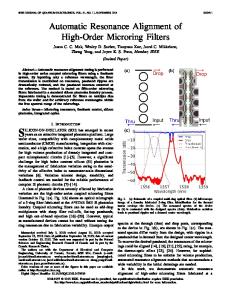
Chapter 1 Introduction Score is a form of musical notation. It is most commonly known as sheet music but can also be presented in a digital equivalent. It is a symbolic representation of music. Each note to be played by the musician is described in terms of its pitch and playing characteristics. The relative position in time and length of each note are also recorded. Relative timing is specified by the tempo, i.e. the speed at which the musical piece should be played. The tempo may vary from one part to another but it is usually steady across one or more sections of the piece of music. While tempo may be specified as a constant for a longer part of the piece it is often idealistic. It hardly ever reflects the reality of a human playing. And it is most certainly not the case with live performances or recordings made without a reference track. In fact, software synthesisers that attempt to mimic human playing often tend to loosen timing and velocity of individual notes to convey realism. There are, however, many applications in which the opposite process is required. That is, having a music recording and the corresponding score, obtain the best match between the two (Figure 1.1): 1. In film and music industries, session musicians are often given the score to the music they are to record. Once recorded the results of an alignment may be used to guide or aid the process of error correction with little or no intervention required. 2. In musicology the score with automatically marked tempo may be invaluable for performance analysis and evaluation. An example would be the comparison of the interpretation of the same musical score by two or more musicians.
1
Figure 1.1: Goal of score alignment. The upper graph is a valid transcription of the original audio in the lower graph, misaligned in time and possibly in tempo. The selected notes at about 24s in the score occur at about 26s in the audio. 3. In computer science indexing or segmentation of continuous media can be used for creating a database for subsequent model training and content-based retrieval. The former exploits the machine learning techniques to improve music transcription or speech recognition. The latter attempts at finding the database entries that best mach the musical or symbolic data supplied. 4. Professional and amateur musicians may benefit from the new capabilities while working with their scores in music notation software. The score can be auditioned by playing back a prerecorded track synchronised appropriately. The work presented here attempts to approach to the last application on the list. While the methods are similar to the first three examples, the goals have subtle differences. It is probably beneficial for the first three tasks that the alignment is ground-truth, possibly with some automatic error detection functionality. The present application on the other hand, is targeted towards a non-technical user. It may seem logical to responsibly cover up the errors in the alignment to improve the perceptional alignment quality. Such problems include both the errors resulting from alignment, as well as the mistakes in transcription or performance: 1. The alignment process may be confused by the musical content and produce incorrect results in the short periods of time, usually in the transition between two sections, like verse and chorus. This may be caused, for example, by the drummer going hard on drums or expressive vocals not being reflected by any instrument in the score. 2. While this is not an error, but rather something to be wished for in other applications, a high alignment resolution causes the tempo to always change from one note to another. 2
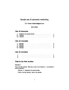
Should the audio recording be time scaled to reflect every small change in tempo, it will loose its human touch and will be unpleasant to listen to. Added to that is a noticeable loss in quality introduced by changing the playing rate so often. 3. The score may introduce repeated or be missing sections, usually due to incorrectly transcribed song structure. One of the main research goals has been to account for the first two of the above problems. Obviously, it introduces certain constrains on the types of music that can be processed. But perhaps only music in highly experimental styles will be misinterpreted by the improved algorithm. Usually when there is a sudden change in tempo, it is kept constant across longer periods of time before the next change. Another important aspect of the problem is its computational complexity. The algorithms widely used to solve alignment problems require long running time. To give an indication, an unoptimised solution takes over 20 seconds to align a 4 minute song with its score. This is undesirable for a casual user and can be reduced considerably. Several optimisation solutions have been studied and a proposal developed. To reason about the design choices made, the discussion will follow with reference to a notation editing software TuxGuitar (Figure 1.2). The program is targeted at guitar players but can be used by all musicians for the purposes of editing and viewing scores. It currently allows playing back the score through several software synthesisers approximating the sounds of real instruments. It supports third-party extensions so one can be built to include the functionality described here. The extension would allow importing an audio file into the software. Subsequent use of the transport control buttons (play, next bar, loop, etc.) will result in the imported audio file being played from the appropriate position. This would allow musicians to play along to the original studio recordings or backing tracks freely available on the Internet, while at the same time visualising the scores to be played. The current progress of this extension development will be discussed in the Implementation chapter of this document.
3
Figure 1.2: Main window of TuxGuitar, a guitar tablature and score editor. Plays back the scores, graphically following the position in the song. The following section will cover the theory and the main alternatives proposed by researchers in the field. The technical details of the author’s system will then be disclosed. The report will be concluded with the evaluation results and a discussion of the next steps to the system.
4
Chapter 2 Background The core of system to be developed can be divided into three main subsystems: Feature Extraction, Alignment and Error Correction (Figure 2.1). The inputs to the system are an audio and a score (also in form of audio, synthesised from MIDI, to be introduced). Two outputs are expected: 1. The original audio, time scaled to sound in sync with the score. 2. The alignment map, i.e. a plain text file containing mappings from sample indices in the original audio to their new positions when time scaled. This section discusses the main approaches in the field of score-to-audio alignment and their relevance to the problem at hand.
Figure 2.1: Preliminary overview of the system. Includes Feature Extraction, Alignment and Error Correction subsystems.
5
2.1
Feature Extraction
Score and audio fundamentally differ in the ways they are represented in data and content they carry. Musical Instrument Digital Interface, or MIDI for short, is an implementation of the score in digital systems. It is a protocol for communication between electronic musical instruments, devices and computers. It defines a notion of events which, along with other control structures, can represent the notes and their characteristics. The latter include instrument, pitch, duration, velocity and basic playing techniques. The methods described in this document are applicable to any digital score representation that gives access to pitch and timing information of individual notes. However, since the target system uses a representation similar to MIDI, the terms MIDI and score will be used interchangeably. While score is a purely symbolic representation of music, a valid audio signal is continuous by nature and carries enough information to reproduce the music as intended. It is a digital signal represented as a bitstream of amplitude quantities, called samples (Figure 2.2). The samples are captured at equal intervals Fs times a second, thus Fs is called the sampling frequency or sampling rate (e.g. 44100 Hz).
Figure 2.2: Waveform of stereo digital audio signal. The frame contains a zoomed in fragment, where individual samples are distinguishable (blue dots). Due to the differences described above, Audio and MIDI cannot be compared directly. A common representation of inputs is needed. Two main options have been explored by researchers and discussed below are: • alignment in symbolic domain, and, • alignment based on audio features.
6
2.1.1
Symbolic Domain
Digital music analysis in symbolic form has been used long before the computers became powerful enough to manipulate digital audio. Such a symbolic alignment method implies transcribing the given audio into MIDI and performing alignment between the transcribed and original MIDI representations of the same musical piece. The approach has its advantages: 1. Partial but reliable transcription will suffice. This means that once the main melody notes, chord changes and basic rhythmic structure are transcribed, the alignment will most probably succeed. The transcription algorithm does not need to pick up every little detail to obtain a high quality alignment. In fact, a few researches have shown that it is enough to guess the note onsets and the pitches of notes [3], [4]. 2. A precise transcription will guarantee a precise alignment. If onsets of the notes are determined correctly the match would be exact around these notes. However, it may be problematic to detect the exact time when the note started. Among the disadvantages of the approach is the general difficulty of the of polyphonic audio transcription. It is a research area on its own. While there has been some success in the field, it is generally considered an unsolved problem. The methods that exist normally introduce constraints on the input audio. So the alignment is highly dependant on what the transcriber can and can’t detect (e.g. support for polyphony, drums, multiple instruments with a similar timbre, etc..) Some interesting works using this approach include the work by Müller et al. [3]. Their system was claimed to be able to align piano music of arbitrary complexity and genre. They made use of the fact that the characteristics of piano sound are well known. This made it possible to detect note onsets for each of the 88 piano keys with a high degree of reliability. They did not provide any numeric evaluation of their results except time and memory measurements. However, the results of several alignment experiments have been made available online. The system performed accurate alignments of examples that included complex jazz and classical music. The restrictions imposed on the music that can be aligned were too narrow to choose this method the target application.
7
2.1.2
Audio Domain
As an alternative to a complicated and generally restrictive method of aligning in symbolic domain, a diametrically opposite technique was researched and successfully employed. Audio is generated from the given score and the alignment is performed between the original and the synthesised audio. This method is fairly permissive as it allows some instruments to be missing from either the audio or the score. Similarly, vocal tracks may be substituted by an instrument track in MIDI, or often omitted all together. It works to a high degree of acceptability on more genres without further optimisations, thus increasing the probability of a successful alignment. In many cases audio transcription is purely programmatic task not requiring any training data. Audio synthesis, on the contrary, may require prerecorded data to be distributed with the application. This introduces overhead to the distribution size (1-20 MB). This may be negligible in other software packages, but TuxGuitar, the target system, is available as a Java WebStart Application. The executable may be downloaded and started in a convenient way from any Internet enabled computer. Therefore the footprint size of the system should be monitored to insure this compatibility. In regards to the distribution size constraint [5] has been helpful. They have looked at three possible ways to generate audio from MIDI that work with different degrees of accuracy: 1. A full-polyphony audio is likely to be similar to the original audio. It is obtained by substituting the MIDI note events with prerecorded instrument samples. The smallest of such libraries are typically 10-20 MB in size. 2. Using piano or another instrument samples for every instrument in the MIDI was shown to have little impact on the quality of the alignment. This is due to the fact that the emphasis here is on the pitches and chords rather than timbres of individual instruments. It adds little overhead to the distribution size (less than 1 MB). Percussive instruments (e.g. drums) cannot be substituted by a pitched instrument (piano, strings, etc.), of course. 3. When chroma representation is used (to be discussed later) the previous approach can be taken further. Simplistic data is generated directly from MIDI to reflect the pitch information only. This is very efficient and requires no sample libraries to be supplied. In the referenced work it was said to have had little impact the results, even though it ignores some of the information that would otherwise be present in the synthesised audio 8
(e.g. harmonics).
2.1.3
Spectral Features
It is clear that alignment in audio domain is more suitable for a general, widely applicable solution. However, it is not that easy to define a good metric for similarity even between two audio files. In Figure 2.3 waveforms of chords C and Fm7 taken on a guitar are shown in the top row. One can see changes in amplitude over time: there is a fast attack with an immediate transient, after which the signal starts rapidly decaying. However, there is not any pitch information that would distinguish the two chords. It would be very hard if not impossible to align two complex pieces in this 2 dimensional representation. On the other hand the required information may be retrieved when working in the frequency domain, essentially adding a third dimension. The spectrograms of the same C and Fm7 chords are shown on the bottom row. Spectrograms are plots of energy of frequency ranges over time. Fundamental frequencies of individual notes and their harmonics are detectable. Two audio clips appear to be different.
a.
b.
c.
d.
Figure 2.3: Time vs. Frequency Domains. (a) Chord C waveform. (b) Chord Fm7 waveform. (c) Chord C spectrogram. (d) Chord Fm7 spectrogram. Any time series including digital audio signal can be converted to frequency domain using Discrete Fourier Transform (DFT). DFT expresses the signal as a sum of sinusoids scaled and phase-shifted appropriately. Individual frequency components of the original signal are found along with their relative amplitudes (Figure 2.4). The spectrogram of a signal is therefore a successive application of DFT to a sliding window of adjustable size, showing spectra of the signal varying over time. 9
3
1
2 si n(2π
+ si n(2π
16 F sn )
0.8
1
Amplitude
Amplitude
2
4 F sn )
0 −1
0.4 0.2
−2 −3
0.6
0
0.2
0.4 0.6 Time(s)
0.8
0
1
0
10
20 30 Frequency(Hz)
40
Figure 2.4: Digital signal in time domain (left) and a corresponding representation in frequency domain (right). The spectral representation is demonstrated as an appropriate for the inputs comparison. It is now possible to define a measure of similarity between two audio frames. The output of DFT is a vector of DFT bins, containing the amplitudes and phases of the sinusoids making up the signal. This means that standard vector distance measures may be applied. Some of the options are: • Cosine distance (employed in [1])
da,b =
aT b kakkbk
ranging [−1, 1] with higher values of d expressing a higher similarity between a and b. • Euclidean distance in n-dimensional space (employed in [2])
da,b
v u n uX = t (ai − bi )2 i=1
ranging [0, ∞) with lower values of d expressing a higher similarity between a and b. The choice of a formula between Cosine and Euclidean distance is not likely to impact the quality of the alignment in any way.
10
2.1.4
Chroma Features
The direct comparison of two DFT vectors is only one possible measure of similarity of two audio frames. A number of researchers [2], [5], [6] have successfully used the concept of discrete chroma vectors as audio features. The output from DFT is in the frequency domain where frequencies of musical notes are well known. The 12 pitch classes (C, C#, D,...) recur every octave, so each DFT bin is assigned to the nearest pitch class as shown on Figure 2.5. The magnitudes are averaged within each bin. The set of 12 bins is called a chroma vector. A sequence of chroma vectors therefore constitutes a chromagram. There are a few immediate advantages to this approach: • Vector size is reduced to 12 elements (as opposed to 1024-8192 depending on the window length in the case of pure DFT). Calculating vector distances becomes considerably more efficient • It is also a more music oriented approach since it is sensitive to pitches and chords • Although it may seem like a disadvantage that the same notes from different octaves are mapped to a single bin; it has been shown by researchers that this performs well and it is appropriate to focus on pitch classes and ignore timbre of individual instruments. In fact, chroma vectors are insensitive to spectral shape • As it was discussed among other audio synthesis options, chroma vectors can be generated directly from MIDI events by mapping a value of 1 into the chroma bin corresponding to the note’s pitch class. To take into account the velocity parameter the value may be scaled. This form of chroma vector generation is not entirely justified since not all of the harmonics return into the same bin as the fundamental frequency However, it has been confirmed by Ellis [11] that chroma content rarely changes within a single beat. Both [10], [11] have used chroma vectors in conjunction with a beat tracking algorithm thus allowing longer windows to be used. This suggests that the chroma features alone may not be enough to produce an alignment at high resolutions and may not replace the method based on spectral features.
11
Figure 2.5: Piano keyboard with approximate frequencies marked. Every frequency range corresponding to pitch class E is mapped to the same chroma vector bin.
2.1.5
Summary
This section (3.3) has covered the literature on previous work relevant to the feature extraction stage. Alignment in symbolic domain has been discarded almost immediately due to its complexity. Alignment based on audio features offered flexibility and proved to yield good quality alignments across a broad selection of music genres. The synthesis method to be used has to be a trade-off between quality and distribution size, with a bias towards quality. The audio features to be extracted from audio can be a spectrogram or a chromagram. Both methods were attractive and needed to be evaluated side-by-side.
12
2.2
Alignment Stage
Once the audio features are extracted, the alignment subsystem can use them to perform the matching process. There are a few techniques for finding the best match between two data sequences. The ones encountered most often in the works on score-to-audio alignment are Dynamic Time Warping (DTW) and Hidden Markov Models (HMM). The latter has been discarded due to it complexity and the requirement for model training. In fact, in [7] HMM was only applied after a preliminary DTW alignment. This ensures that the notes are already mostly aligned and thus no pitch information had to be encoded into the HMM. The technique is based on the notion of state transition where, for example, in sung voice the possible states are transient, silence, steady state (actual body of the word) and breathing (Figure 2.6). Some states are more likely to be followed by other states and some transitions may be prohibited.
a.
b.
Figure 2.6: a) Four-state basic state sequence: silence (S), breath (B), beginning transient (BT), steady state (SS), end transient (ET) and possible transitions between these. b) Time domain representation of a sung note with the HMM states labeled. Transition probabilities may be calculated from manually labelled audio. This requires distributing the training data with the application as well as crafting the model suitable for many genres of polyphonic and polyinstrumental music. It was therefore decided to focus on a more generally applicable Dynamic Time Warping technique.
2.2.1
Dynamic Time Warping
Dynamic time warping (DTW) is an algorithm for finding the best match between two time sequences which may vary in time or speed. With certain additions it has been used successfully for spoken word recognition [9] where a string of words is matched against a set of reference patterns of individual words. However, its use is not limited to applications in signal processing as long as the two time series have a defined metric of similarity between any two of their elements. 13
In its simplest form the algorithm is a typical example of dynamic programming problem solving method. The calculations are performed on a matrix which is commonly referred to as similarity matrix. The row and column indices of a similarity matrix are time frame indices into the original and synthesised audio respectively. The frames, possibly overlapping, are audio features extracted from the audio in that time range as described in the feature extraction section. Each element SM (i, j) of the matrix is a measure of similarity between ith frame of original audio and jth frame of synthesised audio. Similar frames are represented visually as darker spots on Figure 2.7. A dark diagonal path represents the best match between the two audio and is therefore the desired result of the alignment algorithm.
Figure 2.7: Similarity matrix using spectral representation as the audio features. DTW runs on the similarity matrix as its input. Each element DT W (i, j) is the cumulative distance along the best path from (0, 0) to (i, j). The algorithm is based on the observation that if cell (i, j) belongs to the lowest cost path across the whole matrix, then that path contains, as part of it, the best path from (0, 0) to (i, j). It is therefore possible to reuse the results from previous calculations to determine the next step. More precisely, for every element (i, j) several
14
a.
b.
c.
Figure 2.8: Examples of DTW neighbourhood patterns. Marked cells are examined as best previous steps on the path to (i, j). neighbouring cells are considered. The best paths from (0, 0) to those cells are already known making it possible to choose one with the minimum cost. That cell becomes the second last step along the best path to (i, j). The neighbouring cells considered at each step are defined by the pattern which may be customly designed for the application. The pattern on Figure 2.8a is the simplest and the only one of the three presented that allows skipping the whole sections of one or the other audio (by going vertically or horizontally). The formula for calculating the cost of best warp path to cell (i, j) is as follows: DT W (i − 1, j) DT W (i, j) = min DT W (i − 1, j − 1) DT W (i, j − 1)
+ SM (i, j)
(2.1)
In many cases this properly handles the missing or extra notes as well as incorrectly transcribed song structure. The other two options require at least one move in every direction at each step. As a workaround [1] presented a two stage algorithm. DTW is first applied using a pattern similar to 2.8a. Any sections with dominating vertical or horizontal moves will then be removed from the respective audio. The algorithm will be run again this time using pattern 2.8b (Figure 2.9). Pattern 2.8c has been used in [4] in an attempt to obtain smoother transitions right out of DTW. While this would achieve excellent results in many applications, it still only allows 5 discrete directions at each step. This would imply that the direction of the path would be constantly changing when the ideal direction is anywhere between them. If the changes occur too often, noticeable quality degradation of time scaled audio will most probably be introduced. It is therefore might not be possible to carefully model smooth paths having longer sections of constant tempo with DTW alone. 15
Figure 2.9: Two-stage alignment. White rectangles indicate the diagonal regions passed to the second-stage alignment (note the flipped direction of the vertical axis). It should be noted that DTW only produces the cost of the best path through the matrix. As the dynamic programming style might suggest a simple backtrace from the last cell to (0, 0) will return the best path as a sequence of frame indices of the two audio.
2.2.2
Optimisation Techniques
DTW always returns the optimal path and was shown to perform well. It runs in time O(n · m) where n and m are the number of feature frames of original and synthesised audio respectively. For simplicity the length of both time series will be assumed to be n, so the asymptotic behaviour becomes O(n2 ). Given a 4 minute song and the window length of 128 milliseconds (overlapped by half), which is indicative of the real values used with the system, the number of frames in each song is 3750. This results in a similarity matrix with over 14 million cells in it and takes a total of about 20 seconds running time on a 2.67 GHz machine in the MATLAB environment [21]. Increasing the length of the song to only 5 minutes, which is not uncommon either, results in a 31 seconds running time confirming the quadratic asymptotic behaviour. This is not desirable considering that most of the audio used with the end product will probably be very close to the score and only minor tempo modifications will be required.
16
a.
b.
Figure 2.10: Two DTW constraint models: (a) Sakoe-Chiba Band and (b) Itakura Parallelogram. In both cases only the shaded cells are evaluated. Methods used to make DTW faster fall into three categories: 1. Indexing 2. Constraints-based 3. Data Abstraction 1. Optimisations in the indexing category attempt to reduce the number of times DTW has to be applied when a set of time series is given. An example of such a problem would be finding in set of time series one that is more similar to a given time series than the others. This relays back to the example of connected word recognition in [9] which could potentially employ the optimisation. As for the problem at hand, further research could be done that would take into account the repetitive nature of music. It may indeed be possible to convert it to a problem which would benefit from indexing optimisations. However, this is out of scope of the current research. 2. Constraints-based optimisations reduce the running time of DTW by limiting the cells that are evaluated in the similarity matrix (Figure 2.10). Such a constrained algorithm will produce good or even optimal results in most cases where the score is a correct representation of audio. It may fail, however, when the score only partially represents the audio track. Suppose, the imported recording is a cover of the original song by another band and there are new sections introduced that are not in the score. Then the horizontal parts of the otherwise optimal path may be clipped by the boundaries of the constrained region.
A more adaptive constraint model, Path Pruning, has been used in [4]. For every successfully evaluated row in the cost matrix the paths with the augmented cost lower than 17
a specified threshold are selected. The leftmost and the rightmost of such paths become the boundaries for the corridor in which the next row is evaluated. The threshold is dynamically calculated and is a function of the best cost encountered in the previous row. Such a model is designed to easily adapt to movements in the vertical direction and with sufficiently large threshold - in horizontal, too. 3. Data abstraction based optimisations focus on the idea of performing DTW on the reduced representations of data. That is, performing DTW at a lower resolution, then working up to higher resolutions as required. In the case of the problem at hand this would mean taking larger frame sizes and using the results of DTW as an approximation for further DTW applications. An innovative method has been proposed in [8], that combines the constraint-based approach with data abstraction achieving linear runtime and memory requirements. The algorithm, FastDTW, proceeds by recursively reducing the resolution of the time series by a factor of two, applying DTW at a lower resolution and using the resulting path to constraint DTW at the next finer resolution (Figure 2.11). Although the algorithm may seem very attractive, it will not be able to improve the performance of score-to-audio alignment. Since it requires creating a reduced data representation at every resolution (O(log n) times in total), introducing computational overhead, it only significantly outperforms plain DTW when the length of the time series exceeds about 10000 elements. This is about twice as many elements as needed for a good time resolution for an average length song.
Figure 2.11: The four increasing resolutions evaluated during a complete run of the FastDTW algorithm.
18
2.2.3
Summary
This section (2.2) presented an overview of the literature for the problem of aligning two sequences containing extracted audio features. The two alternatives were Hidden Markov Models and Dynamic Time Warping. The former was discarded for the reasons of complexity and because it required distributing model training data with the software package to the end-user. On the other hand DTW proved to be a good algorithm for this task. Several DTW movement patterns were considered. The simplest of them offers two orthogonal and one diagonal movement at each step (Figure 2.8a). Even with the simplest model there were concerns regarding the poor DTW performance time-wise. Several optimisation techniques have been reviewed. Some did not seem to meet the requirements of the software (like statically constrained methods), others did not improve performance in the case of the current task (FastDTW) or were simply inapplicable to the problem (Indexing-based approaches). One improvement that did seem suitable was the adaptive constraint based approach, where the corridor for the warp path is determined dynamically.
19
a.
b.
Figure 2.12: DTW artifacts: (a) minor path inconsistencies and (b) path direction limitation
2.3
Error Correction
One of the outputs of the proposed system is a time scale modified audio. This means that the audio produced will be time stretched or compressed to adapt to to the tempo of the score. There are, however, several problems associated with this requirement that arose with the use of the Dynamic Time Warping algorithm introduced previously. • DTW often returns a “bumpy” path in the parts of the song where several consecutive frames are similar to each other (Figure 2.12a). • DTW returns a numerically optimal path which does not always coinside with the musically correct alignment (e.g. as above) • A careful listening test showed that minor but frequent playback speed changes introduce a noticeable quality loss • If the warping path produced by DTW is interpreted directly, the only playback rates would be 1, 0 and Infinity introducing discontinuities in the music (Figure 2.12b). It was therefore crucial to investigate possible ways to keep the tempo constant across longer sections of an audio file. Most of the works studied in the scope of this research only aimed at producing the appropriately modified score that would sound in sync with the audio. Surely, the modified score can be re-synthesised and would not have the problems of the time scaled audio. 20
While [1] was one such research, they did look into addressing some of these issues. In addition to applying a two-stage DTW mentioned previously (Figure 2.9), the path was smoothed across multiple alignment frame pairs. However, no discussion of the smoothing method was provided. The remainder of this section is devoted to discussing several smoothing and fitting techniques from mathematics, statistics and computer graphics.
2.3.1
Requirements
It is important to establish the requirements to the error correction algorithm as well as its inputs and expected outputs. Ideally the algorithm would be able to analyse the path and segment it such that the slopes of the segments are piece-wise constant. Given a threshold in milliseconds, the segments should be the longest possible such that the new position of each point is within the threshold distance from the path predicted by DTW. The path would be supplied in the form of frame pairs which can be treated as Cartesian coordinates in two dimensions. The expected output is a reduced number of coordinates, called knots, such that the linear interpolation of these approximates the warping path according to some predefined metric. Sample input and output are illustrated on Figure 2.13.
Figure 2.13: Automatic segmentation detection. Warping path as returned by DTW (blue) and detected segments (red).
2.3.2
Curve Fitting
A major area of study that has been looked at was curve fitting. Curve fitting is the process of constructing a function that has the best fit to the given data. It may either be an exact fit to the data (also called interpolation), or approximate (smoothing). • Interpolation is inapplicable since the warping path is already defined by a large number 21
of points. However, the output of the algorithm, i.e. the sequence of knots, is linearly interpolated to produce the new path. • Smoothing is the process creating an approximating function that attempts to capture important patterns in the data, while leaving out noise or other fine-scale structures. This definition very closely resembles the problem at hand. In many cases, the warping path is already a straight line, distorted by some off the line bumps. Many smoothing techniques are inapplicable due to the nature of the input data or the expected output: • Some are targeted at processing a set of observations of some real world variables that form a relationship, yet are scattered around some unknown points being approximated. On the other hand, DTW model precisely defines the relative positioning of two consecutive points on the path (Figure 2.8). • Besides, the smoothing may be carried out based on purely local features and does not guarantee any functional relationship on the output data (e.g. polynomial, or, in the present case, piece-wise linear). To preserve the focus on the linearity of the output the research was turned towards the smoothing methods that employ linear regression discussed below.
2.3.3
Linear Regression
Linear regression is a technique to model a linear relationship between two or more variables. To relate it back to the original problem, suppose that the abscissas and ordinates of all of the points in the warping path form vectors X = x1 . . . xn and Y = y1 . . . yn respectively. Also suppose that the path is conceptually a straight line. Two points is sufficient to uniquely define a line, yet there is n of them it total. Such a line is said to be overdetermined. Thus it is not possible to uniquely fit a line y = ax + b through points (xi , yi ) where i = 1 . . . n. Proceed by introducing an error parameter ε and solving equations yi = axi + b + εi , while minimising ε in some way. The least squares method approaches it by minimising the sum of squared errors: 2
kεk =
n X i=1
ε2i
n X = (yi − axi − b)2 i=1
22
(2.2)
But kεk2 is a quadratic function of a and b, whose minimum is reached when both partial derivatives are 0: n
X ∂kεk2 = −2 xi (yi − axi − b) = 0, leading to ∂a i=1 Pn
i=1
xi
n
Pn a+b=
i=1
yi
n
, and
(2.3)
n
X ∂kεk2 (yi − axi − b) = 0, leading to = −2 ∂b i=1 P P xi xi y i i a + P 2 b = Pin 2 i xi i xi
(2.4)
The system of two linear equations 2.3 and 2.4 can be written in matrix form as
P
i
xi
n
1
1 P x P i 2i i xi
a b
=
P
i
yi
n P xy i P i2i i xi
This can be rearranged to find a and b as follows: P P P n x y − x y 1 i i i i i i i P = P P P P P 2 2 2 x ) x − ( n i i i i b i yi − i xi i xi y i i xi
a
(2.5)
The coefficients can be substituted back into 2.2 to give the equation for sum of squared errors (SSE ) or alternatively mean-square error M SE = n1 SSE. MSE can give an idea of how √ good the model is on average. Recalling the original problem, M SE is actually the average vertical distance in frames, between the fitted line and the warping path as returned by DTW. By using linear regression it is possible to fit one straight line to the compete data set. However, due to the possible tempo fluctuations between the two inputs, it is required that multiple lines are fitted. Below are some of the possible solutions that use linear regression in conjunction with the least squares method. Local Linear Regression Smoother, first introduced in [16], starts by fitting a regression model to the data within the window of some predefined size λ sliding by ∆X. The estimate for the mid point X0 of the window and its neighbourhood is a constant equal
23
Figure 2.14: Application of local linear regression smoother. The result estimate Yˆ (X0 ) is the value of the fitted line at X0 (black). to the value of the fitted line at X0 (Figure 2.14). The process is repeated for every X0 by shifting the window by ∆X. This is a greedy algorithm which does not need the complete data set to operate. It is very efficient and may be applied to the warping path with the following remarks: • The window must be sufficiently large (and the overlap sufficiently small) to actually cure the problem of continuously fluctuating tempo • Larger window, on the other hand, adapts more slowly to the real tempo fluctuations, thus may introduce discrepancies in the sound, defeating the purpose of error correction • The window and the overlap parameters are fixed for the run of the algorithm and cannot be set according to the desired mean-square error threshold in advance.
Multivariate Adaptive Regression Splines, abbreviated as “MARS” [17], is an extension of linear models which automatically determines the knots from the provided data and returns a set linear function providing the best fit between the corresponding knots (Figure 2.15). It proceeds in two stages: 1. In the forward path it iteratively searches for the knots which, when added, give the maximum reduction in SSE (sum squared error). The search is stopped when either 24
Figure 2.15: Application of Multivariate Adaptive Regression Splines method modelling the relationship between two variables. The fitted model (black) has five knots at about 0, 1.5, 3.3 4.7 and 6. the change in the overall SSE is negligible or the maximum number knot is reached (user-adjustable parameter). 2. The backward pass prunes the model by removing the least effective knots until it finds the best submodel. The algorithm trades off fitting quality against model complexity and no longer uses pure SSE as the criteria for choosing the candidate knot to be pruned. MARS method automatically partitions the provided data into sections with one linear model in each of them without making an assumption about the length of such sections. This seems especially relevant to the problem of audio-to-score alignment where it is difficult to predict the number of places of tempo fracture in advance. The algorithm allows adjusting the maximum number of knots and various other limits, which may appear to be useful for the problem at hand. Indeed, the User may want to take over the system and manually control the error correction. This might as well cure some particularly bad alignments by smoothing things out. However, it is not clear how well it performs on the data which is already mostly in linear relationship and the tempo changes are very subtle. Never-the-less, this technique provides a good motivation for further research and demonstrates relevance to the problem at hand.
25
2.3.4
Summary
A range of methods for smoothing the warping path and correcting the DTW errors have been presented in this section. The most relevant ones to the problem at hand were based on linear regression. The discussion forms the mathematical basis for the respective section of the proposal. It presents the theory behind the linear regression using the least squares method and derives the necessary formulae for its application.
26
Chapter 3 Proposed Solution This section covers the details of the proposed system at a conceptual level with only some implementation details. It presents design decisions at every step (Figure 3.1). Several parts of the system offer more than one alternative implementation so as to aid evaluation by comparison.
Figure 3.1: Overview of the system with chosen alternatives at each stage.
27
3.1
Target System
The alignment method proposed in this document was designed with a particular target system in mind. It was chosen to be an extension to a notation editing software with playback capabilities. No closed source products were considered as they typically do not have means for extending their functionality by third parties. Two guitar players oriented open source software solutions were considered: TuxGuitar [18] and KGuitar [19]. At the time of writing KGuitar is still in alpha development stage. TuxGuitar, on the other hand, is a mature cross-platform software with a large user base. Thus, TuxGuitar was chosen as the target system. TuxGuitar, among other functionality, supports importing scores in various file formats including MIDI. Multitrack scores can be viewed, edited and auditioned using the operating system’s or third party software synthesisers. TuxGuitar is implemented in the Java programming language and can be extended through the use of plugins. It previously did not provide support for importing or playing audio files. Nor did there exist a publicly available audio time stretching library with Java bindings. Developing such an extension has appeared to be time consuming and therefore has not been completed. Besides, the alignment method itself is not yet suitable for use by the end-users. The current state of the implementation will be discussed in the next chapter.
28
3.2
Prototyping Environment
While the final product is designed to extend TuxGuitar’s functionality, the latter had no preexisting support for audio files or basic signal processing routines. To speed up prototyping, Matlab [21] environment was chosen for its scripting features and its substantial digital signal processing support. Also Matlab’s ability to generate complex plots to visualise results turned out to be invaluable. Not all of the system’s features are present in the prototype. As such all MIDI file handling was omitted. Instead, it expects another audio file, which may have been synthesised from MIDI. Generating audio from MIDI is done manually and has only been automated in the TuxGuitar implementation. This also allowed the author to conduct tests by aligning the original studio recording with a backing track or a cover by another band.
29
3.3
Feature Extraction
The feature extraction subsystem focuses on transforming the score and audio inputs into directly comparable structures. Comparison based on audio features has been chosen over comparison in symbolic domain due to the high complexity of the latter. Thus, the score is rendered to audio using a software synthesiser and alignment between two audio is carried out. As discussed before there are two common ways of generating audio for the purposes of feature extraction: 1. MIDI tracks can be substituted by their corresponding instruments, or 2. one instrument can be substituted for every track. Both options were chosen to be implemented since adding support for one when the other is in place did not pose a problem. The third option dealing with direct extraction of audio-like features from MIDI events was omitted as it requires MIDI events manipulation at a low level and was not a priority of the research. Next after the audio is generated, audio features are extracted. Two audio features most commonly referred to in literature were chosen: 1. Spectrograms - created by applying DFT to a moving window with an overlap 2. Chromagrams - created from the spectrograms by adding together and averaging the energy bins around the 12 pitch classes (as described in 2.1.4) The first features preserve the spectral shape of the audio which may confuse the alignment in cases where the two audio are very different in that respect. The second features minimise the differences in spectral shape, focusing on pitch alone. This was found to aid the alignment of pitched instruments but did not honour so much the percussive instruments. Both methods were evaluated against music in various genres. The spectrogram window is of Hann type (Figure 3.2) which is applied to the audio signal through multiplication prior to taking the DFT. The window function is usually applied in order to minimise the effect of the overlap. If the audio is downsampled to 8000 Hz, the highest chromatic pitch present in the transform is B7 at 3951 Hz. This leaves out only one pitch on the standard 88-keys piano keyboard, that is C8 at 4186 Hz1 . In practise the playing range is much lower and the higher octaves only 1
The frequencies are given assuming the middle A to be 440 Hz (ISO 16:1975).
30
Figure 3.2: 64-point Hann window in time domain. contain the smeared higher order harmonics. It is in the interest of the system to remove from the signal as much of the non-pitch information as possible. Another advantage of such a setup is that there are less DFT bins for the same timefrequency resolution. Assuming the sampling frequency of 8000 Hz and a window length of 1024 samples, the time resolution is 128 milliseconds. This almost exactly corresponds to a 1
/16 note length in tempo 120 BPM (Table 3.1). Introducing the overlap with an appropriate
window function, the time resolution is improved further. In practise resolutions considerably higher degrade the quality of the alignment due to the decreased frequency resolution. On the contrary, lower time resolutions often match or outperform it. Tempo, BPM 90 120 150 180
1
1 1 1 /4 note /8 note /16 note /32 note samples ms samples ms samples ms samples ms 5333 667 2667 333 1333 167 667 83 4000 500 2000 250 1000 125 500 63 3200 400 1600 200 800 100 400 50 2667 333 1333 167 667 83 333 42 Table 3.1: Note lengths at 8 kHz sampling rate.
Decreasing the time resolution sometimes comes at the price of minor tempo floating. On careful listening one may hear the percussive hits being slightly off when both tracks are listened to side-by-side. However, this is a reasonable trade-off for performance once the system is used as intended. That is, the User is only hearing one audio track while the position in the song is being visually traced on the note staff. According to a non-official Stanford study referenced in [15] the sound can come up to 45 ms early, or the picture can be ahead of the sound by as much as 125 ms. 31
3.4
Alignment Stage
Out of the two major methods for aligning two musical sequences only DTW was discussed in detail due to HMM’s increased complexity and storage requirements. As for the type of DTW, no pattern would ensure that the path has the right slope in every case. It has therefore been decided to use to simplest pattern on Figure 2.8a and seek other ways of finding the right slope (discussed Error Correction section). DTW has been implemented in the prototype. It was found however, that the algorithm takes undesirably long time to evaluate the whole matrix at sufficiently high resolutions (examples given previously in 2.2.2). After studying the possible optimisation techniques, one of them has been adopted. Path Pruning [4] has been chosen over the other methods since it allows adapting of the constraint corridor to the path direction changes, thus increasing the chances of getting the optimal path in more cases. It follows the constraint-based optimisation pattern. It was described in some detail in the previous chapter. It does not evaluate the complete matrix but it does require it to be evaluated at full resolution in one go.
3.5
Error Correction
It has been decided to use the simplest 3-directional pattern for Dynamic Time Warping and rely on curve fitting to account for the problems associated with this choice and with the DTW method in general. In particular, the algorithms based on linear regression were considered in order to • smooth out the possible discrepancies in the path, • identify the regions with the constant tempo, and • generate the alignment map with less entries than the number of frame pairs in the path. The list of the methods chosen to be reviewed was in no way comprehensive but it provided sufficient directives and motivation to design a custom method for the task. Some of the highlights of the techniques are presented below: • The Local Linear Regression Smoother traded the smoothness against being able to quickly adapt to tempo variations. The window length and the overlap are the only
32
Data points Fitted knots Rectified overshoots
16
14
12
Y
10 B1
8
B0
A0
6
4
A1
2 2
4
6
8
10
12
14
16
18
20
X
Figure 3.3: A sample run of the proposed error correction algorithm with MSE threshold set to 0.2. controllable parameters which cannot be specified in terms of the desired mean-square error or similar. • The Multivariate Adaptive Regression Splines (MARS) method is a sophisticated algorithm that can automatically determine the most important fracture points in the path (knots) and gives room for manual configuration. It has been decided to design an algorithm specifically for the task, that would address the problems of the fixed-window algorithms yet be simpler and more efficient than MARS. The new algorithm makes use of the fact that the step of the input data is small and non-decreasing (i.e. ∆x, y ∈ {0, 1}). The algorithm is still able to perform adequately on other data, e.g. if the pattern is replaced with a more sophisticated one. The new algorithm proceeds by fitting a straight line to some contiguous subsequence from the path using the least squares method (Figure 3.3). If the resulting MSE is below the specified threshold, then the data sequence being looked at is extended by one point. In case it exceeds
33
MSE the data point added last is discarded and the previous fitted line parameters are used to set a new knot. In the figure example this knot is set to be A0 : fitting to the points up to (7, 5) resulting in a too high MSE, therefore to obtain the knot A0 the line was only fitted up to point (6, 5) of the original data. Once the knot A0 is found a new data subsequence begins to accumulate starting with the last element of the previous subsequence, i.e. (6, 5) onwards. When it is time for a new knot (B0 ), it is known that the new line will be a linear model fitted to data points (6, 5) up to (17, 8). Now that the parameters for both the previous and the current line are known, the algorithm goes back to the previous knot A0 and updates it to be the intersection A1 of the two lines. The algorithm proceeds in this fusion until no data points remain. The algorithm’s pseudo code is presented in Listing 3.1. It currently runs in quadratic time in the length of the path but can easily be made linear by not recalculating the regression model at every iteration. In practise this computational overhead does not pose a problem.
3.6
Summary
This chapter presented and justified the design decisions of the implemented system. It introduced the target system and the prototyping environment mentioning the separation of scope between the two. Then the two alternative feature sets were discussed covering some of the constants involved. The alignment stage was only briefly touched up since DTW was discussed in detail in the literature review section. The implementation specifics are left for the respective chapter. Lastly, a new Error Correction algorithm was presented as an alternative for more complicated DTW patterns. Simultaneously the algorithm takes the responsibility of reducing the number of points in the path for a faster and a higher quality audio time scaling. While this chapter only described the high level design with only some implementation introduced, some of the most important implementation issues and details will be revisited once more in the following chapter.
34
Algorithm 3.1 Error correction algorithm pseudo code. /* * * Fits straight lines to a sequence of data points automatically * determining the knots . The algorithm assumes the presence of * LeastSquares function reterning the slope / intersect of the * fitten line and the resulting MSE . * * path sorted sequence of data points * thresh MSE threshold that * each * line will not exceed * retruns sorted collection of knots */ FitLines ( path , thresh ) // initialise knots = [] // result is collection of points data = [] // window of data from path a0 , b0 = 0 // parameters of the last fitted line foreach point in path data . append ( point ) // add point to subsequence (a ,b , mse ) = LeastSquares ( data ) // fit line to the data /* check if threshold is reached */ if mse > thresh data . remove ( end ) // discard last added point (a ,b , mse ) = LeastSquares ( data ) // fit line again /* first shift the previous knot where it belongs */ x0 = -(b - b0 )/( a - a0 ) // find intersection y0 = a * x0 + b knots . replace ( end , Point ( a0 , b0 )) /* find the coordinates of the new knot */ x = data ( end ). x y = a*x + b knots . append ( Point (x , y )) a0 = a // record the parameters of b0 = b // the just fitted line data = [ data ( end ) , point ] // reinitialise subsequence end if end for return knots end FitLines
35
Chapter 4 Implementation The previous chapters were devoted almost entirely to the design of the system. Textual explanations with some pseudo code additions ware provided for each technique employed. The present chapter builds upon the content of the previous chapter and projects it onto the target system and the prototype. It discusses the interaction between the parts of the system and the external frameworks or systems. Additionally, it elaborates on each technique by describing implementation specific issues that had to be overcome.
4.1
Target System
TuxGuitar, the target system, is a powerful guitar tablature editor enabling guitarists to edit and listen to multitrack scores. It is written in Java programming language around the Standard Widget Toolkit (SWT [20]) to provide native look on all supported platforms. One of the reasons for its popularity is its extensible design. It provides support for extending its functionality through the use of several categories of plugins: Browser Plugins: Extend the built-in score collection management system. They unite the online community resources and the local content. Importer and Exporter Plugins: Add support for new score file types. In fact, MIDI support is provided in the form of such a plugin. These plugins, however, do not extend to audio since audio does not typically contain any score information. MIDI Output Port Plugins: Provide support for more synthesisers to audition scores. It refers to both software and physical output ports. The possibility to audition the scores 36
through the Gervill software synthesiser, discussed earlier, is provided in the form of a plugin too. MIDI Sequencer Plugins: Sequencers are low level implementations for MIDI playback handling. It is discussed in detail below. Tool Item Plugins: General purpose plugins conveniently placed into the application’s menu that have access to all internal structures and functionality. Implementing the plugins falling into the last two categories was needed to get the required functionality into TuxGuitar. The tool item plugin is only useful for providing a simple user interface to the system, allowing to tweak alignment settings and to select an audio file to import. Designing a user interface has not been a focus of this project and thus has not been implemented at the current stage. MIDI Sequencer, on the other hand, is the central point of communication between the alignment system and the host application and deserves close attention. It is responsible for directly receiving the User’s playback commands and delivering each note to the selected synthesiser. Therefore, it is the duty of the sequencer to manage timing of the individual events heard in the output. In return the application expects from the sequencer the current position in the song, which it queries at regular intervals and shows visually on the screen. The task of the replacement sequencer is to mimic the behaviour of the original MIDI sequencer, yet transparently substituting MIDI by audio. The class diagram for the system is presented on Figure 4.1. The class names are prefixed with BT, which stands for Backing Track, the name of the extension: • BTSequencer is the class directly communicating with the playback system of TuxGuitar • BTToolMenuDialog is communicating with the User through the GUI (not implemented) • BTSettings keeps track of the audio files and alignment parameters acting as the means for communication between the UI and the core of the alignment system. Once the alignment is required, BTSequencer requests it from • BTAlignmentManager, which in turn relies on three class hierarchies corresponding to the three main components of the designed alignment system (Figure 3.1): – BTFeatures 37
– BTDTW – BTErrorCorrector To be able to process audio files in various formatas and to unify the handling of audio files and in-memory generated audio • BTStream and BTPlayer classes have been implemented to read and playback audio, transparently converting it to the desired sampling rate. They both heavily rely on the Java Sound API. BTSequencer and BTSettings are described in more detail below deferring the discussion of other parts of the system until their respective sections. BTSequencer implements TuxGuitar’s internal interface MidiSequencer which in turn is modelled after the Sequencer interface of the Java Sound API. It is the central class of the extension. It is a quite large class but the main functionality can be conceptually expressed in the six methods: • start/stop methods are self explanatory • getTickPosition/setTickPosition and getTickLength, despite the slightly misleading naming, actually query and update the position within the song and the total length of the song expressed in MIDI ticks. MIDI ticks is the base unit of MIDI timekeeping • By design, every time the User starts the playback, TuxGuitar supplies the complete song to the sequencer through the call to createSequence. The new sequence of MIDI events is then compared to the one received the previous time (if any). In case there are differences, the alignment may no longer be valid and has to be computed again One other property worth noting is that BTSequencer always keeps a reference to the conventional TuxGuitar’s MIDISequencer (backupSequencer ). This comes useful for two reasons: • The metronome, available in TuxGuitar, is really another MIDI track which must still be played through a conventional sequencer • The User may wish to temporarily disable the audio backing track and preview scores the old way. Switching the sequencers through the internal TuxGuitar facilities would 38
mean unloading the whole extension, leading to the loss of the current alignment and the associated state. Keeping a backup sequencer ready and initialised makes the switching almost instantaneous by transparently redirecting the method calls. BTSettings is the class used extensively by almost every other class in the system. It has been decided to keep the alignment parameters centralised. This reduces the amount of direct communication between parts of the system leading to cleaner and more maintainable code. The class offers facilities for updating and retrieving both the user-adjustable and internally used parameters. For example, the path to the backing track audio file is set by user through the system’s user interface, while the alignmentRequired flag is only set internally when the underlying song or some parameter have changed, possibly invalidating the alignment.
39
org.herac.tuxguitar.player.impl.bt BTSequencer btPlayer backupSequencer alignmentManager sequence createSequence() getTickLength() getTickPosition() setTickPosition(n) start() stop()
BTStream baseStream baseFormat targetStream targetFormat BTStream(file) BTStream(stream) setFormat(format) skip(n) reset() read(floatBuffer, offset, length)
BTToolMenuDialog settings show() BTSettings alignmentRequired btFile format featuresType windowLength windowOverlap dtwType corridorMinWidth mseThresh isAlignmentRequired() setAlignmentRequired(required)
BTFeatures btStream getFeatureList()
BTSpectrogram specgram getFeatureList()
BTChromagram chromagram getFeatureList()
BTAlignmentManager settings alignmentMap btStream synStream setSynStream() getAlignmentMap()
BTPlayer btStream sourceLine stretcher frameZeroMicrosecond getMicrosecondLength() getMicrosecondPosition() setMicrosecondPosition(position) start() stop()
com.bytekino.jRubberBand RubberBandStretcher nativeObjectAddr RubberBandStretcher(...options...) setTimeRatio(ratio) setPitchScale(scale) getLatency() setMaxProcessSize(samples) setKeyFrameMap(map) study(input[], samples, isFinal) process(input[], samples, isFinal) retrieve(output[], samples)
RubberBandOptions ...Option Enums... options toInteger() set(option)
BTDTW btFeatures synFeatures getPath()
BTDTWSimple similarityMatrix costMatrix path getPath()
BTErrorCorrector path knots getKnots()
BTDTWPruned similarityMatrix costMatrix path getPath()
Figure 4.1: Class diagram for the Backing Track extension. Some book-keeping classes, methods and fields omitted.
4.2
Inputs Processing
As discussed in the design chapter, the score-to-audio alignment is performed entirely in the audio domain. Therefore the score must first be synthesised to audio. Moreover, the internal
audio processing is usually done with the audio samples converted to the floating point representation with the values ranging from -1.0 to 1.0. As it will be shown in Output Generation section this data representation is essential for feature extraction and audio time scaling. Lastly, the file with the backing track selected by the User may be in a variety of different audio file formats and encodings which has to be accounted for. To synthesise audio from MIDI, Gervill library [24] has been chosen for a number of reasons: • It is designed to integrate well with Java Sound API, the standard Java framework for sampled audio and MIDI • It is already distributed with most TuxGuitar packages • The tiny size of 224 Kb including an emergency soundbank (version 1.0) allows it to be distributed as part of even the smallest packages TuxGuitar relies heavily on Java Sound API. In fact, one of the two sequencers that come bundled with TuxGuitar simply delegates the main processing to the default Java sequencer. The framework has been very helpful in the handling of audio. It has implicit support for several uncompressed audio file formats such as WAVE and is extensible by third parties to support MP3, Vorbis/OGG, Flac and other popular compressed audio formats. The conversion is done by the respective classes and is presented to the programmer in a convenient AudioInputStream class. Likewise, the required number of channels, sample rate and encoding to be served by AudioInputStream (e.g. 16/24 bit signed/unsigned integers, or 32/64 bit floats [23]) can be specified through the use of AudioFormat. However, while AudioInputStream captures all the coversion details, it still works at a fairly low level. In particular: • It serves data in byte arrays, which means that the bytes have to be combined into the correct primitives by the client programmer • The channels are interleaved meaning that the samples from left and right audio channels of a stereo file are stored together. This is the way they are expected for playback by Java Sound API, but was incompatible with the Rubber Band time scaling framework which expects a separate array for each channel • Resetting to an earlier position within the file or in-memory audio stream is not always supported. However, this functionality is required in several parts of the system:
41
– the same audio file is usually read at least twice: during feature extraction and during playback – the User may wish to revert to an earlier position within the song or enable looped playback of some section To account for these inconveniences the BTStream class was introduced to simplify the audio handling throughout the extension. It allows specifying the desired target format with the data being read directly into an array of floating point numbers. Additionally it provides functions for (de)interleaving multiple channels, and is guaranteed to be able to reset to the beginning of the track, or to any earlier time point.
4.3
Spectral Features Extraction
Calculating spectral features for the backing track and the synthesised score has been implemented in the class BTSpectrogram. The spectrogram is stored internally as a list of float arrays, representing a sequence of feature vectors for overlapping window frames. L i s t specgram = new L i n k e d L i s t ( ) ; The spectrogram is computed by continuously reading audio data into a buffer, extracting spectral features and adding it to the list of feature vectors. Since the windows may be overlapping and going back in time in the audio input stream is computationally expensive, the overlapping part of the buffer is reused from the previous frame. The spectral features are found by taking Discrete Fourier Transform and taking the absolute value of the resulting complex numbers. More precisely, a Fast Fourier Transform (FFT) implementation for Java [22] has been used. The method from the BTSpectrogram class that computes the spectrogram is presented in full in Listing 4.1 The implementation can also normalise the features (frame-by-frame) if the corresponding option is enabled in the settings by the User. This is done by subtracting the mean of the spectral energy across the DFT bins from every bin. The goal of normalisation is to account for the differences in loudness of the two recordings.
42
Algorithm 4.1 Spectral Features Extraction Algorithm in Java. void doCompute () { int len = getSettings (). getWindowLength (); int ov = getSettings (). getWindowOverlap (); boolean normalize = getSettings (). getNormalizeSpectra (); /* error checking and FFT initialisation code skipped */ // stream data will be read into the following buffer float [] buffer = new float [ len ]; // complex number representation for FFT float [] reals = new float [ len ]; float [] imgs = new float [ len ]; int cnt = stream . read ( buffer , 0 , buffer . length ); while ( cnt != -1) { reals = applyWindow ( buffer ); // apply window function fill0 ( imgs ); // imaginary parts are all zeroes fft . doFFT ( reals , imgs , /* inverse = */ false ); float [] spectralEnergy = abs ( reals , imgs ); if ( normalize ) removeMean ( spectralEnergy ); specgram . add ( spectralEnergy ); // add processed window to spectrogram shiftLeft ( buffer , len - ov ); // reuse overlapping part for next win cnt = stream . read ( buffer , ov -1 , len - ov ); // read rest from stream } }
4.4
Chroma Features Extraction
Extracting the chroma features from audio turned out to be more complicated than constructing a spectrogram and involved solving the time-frequency resolution issues. The chromagram construction proceeds in three steps: 1. The spectrogram of the audio is constructed as described in the previous section 2. The chroma weighting map is computed. It assigns each FFT bin to a pitch class 3. The weighting map is applied to the spectrogram to get the sequence of chroma vectors While chroma weighing map is conceptually a table that maps each FFT bin to a pitch class, it does not have a one-to-one correspondence. Figure 4.2 shows one possible chroma weighing 43
Figure 4.2: Chroma weighting map with window length of 2048 samples at 8 kHz sampling rate (left). Zoomed in at first 31 bins (right). map. Every two consecutive grayscale rectangles on the same row represent an octave interval while the sequence of ascending rectangles between them are the 12 semi-tones in the chromatic scale. It can be seen immediately that the rectangles corresponding to the same pitch class grow exponentially in width and the corresponding FFT bin number. This can be inferred from the formula expressing the frequency of one note in terms of the frequency of another note as follows:
f = f0 · 2n/12 , where
(4.1)
f0 is the fundamental (i.e. central) frequency of the reference note n is the number of semi-tones the required note is above the reference note (can be negative) It follows from the formula that, say, the fundamental frequency fA5 = fA4 · 212/12 ≈ 880 Hz taking fA4 to be 440 Hz which is a commonly used value.
44
The FFT bins, on the other hand, are evenly distributed between 0 and the sampling frequency. That is, each bin is centred around the frequency f = fs ·
k , where N
fs is the sampling frequency, N is the FFT window length in samples, k is the 0-based index of the bin ranging from 0 to N − 1. Considering the example on Figure 4.2, each FFT bin spans
fs N
=
8000 2048
≈ 3.9 Hz. However,
as can be seen from the notes frequencies table in Appendix A, the fundamental frequencies of notes below B1 are less than 3.9 Hz apart. This means that the frequency resolution of FFT with these parameters is not enough to uniquely identify the pitch class for lower notes. This is expressed graphically by vertical bars spanning more than one semitone (FT bins 8 to 16). In the above example the described issues do not pose a problem in practise since the consecutive minor second intervals (1 semitone apart) do not occur so ofter in music. And it is still possible to distinguish notes that are over 1 semitone apart except the first three notes (A0 , A]0 , B0 ). However, if the window length is lowered to 512 samples, the “uncertainty” range extends to B 4 , well into the most common playing range of many instruments. Additionally, the first two octaves are blurred and become practically indistinguishable (Figure 4.3). An alternative implementation has been proposed in [12] whereby the signal is re-sampled to a lower sampling rate before taking FFT thus increasing the time-frequency resolution for lower pitches (Table 4.1) but this is left as a possible enhancement. A0 − B3 C4 − B6 C7 − C8 882 Hz 4410 Hz 22050 Hz Table 4.1: Variable sampling rate chroma extraction.
To calculate the chroma weighting map in Matlab, the following steps have been taken by the author: 1. The central frequency for each FFT bin is determined ffthz = (1: nfft -1)/ nfft *( Fs /2) % where nfft = window /2+1 2. The semitone different between every FFT bin and A0 is determined. This may, and for most bins will be a decimal number, since the central frequency of a bin does not 45
Figure 4.3: Chroma weighting map with window length of 512 samples at 8 KHz sampling rate zoomed in at first 18 bins. necessarily align with any note’s fundamental frequency fftsemitones = N * log2 ( ffthz ./ A0 ) % make up a value for bin 0 fftsemitones = [ fftsemitones (1) -1.5* N , fftsemitones ] 3. Determine how many semitones every bin spans binspan = [ max (1 , fftsemitones (2: nfft ) - fftsemitones (1: nfft -1)) , 1] 4. Iterate over FFT bins ranging from A0 to A8 (the actual implementation allows specifying a different range) % find first bin belonging to A0 fst = find ( fftsemitones > -1 , 1 , ’ first ’) % find last bin belonging to A8 lst = find ( fftsemitones < 88 , 1 , ’ last ’) for k = fst : lst % retreive the semitone difference with A0 n = fftsemitones ( k ); 46
% Notes in higher octaves span more frequencies , penalise them scaling = 1.3^ -( n / N ); % should be 2.0 but we are generous 5. Find the “exact” notes in the neighbourhood of the current bin (since the current bin is most propably somewhere in between two notes). Then assign how much weight the current bin has on each of them % Each semitone is associated with a Gaussian distribution % That is 2* stddev = 1 denom = -2*(1/2)^2; % The note on the left n0 = floor ( n ); M ( mod ( n0 , N )+1 , k ) = exp (( n - n0 )^2/ denom )* scaling ; % The note on the right n0 = ceil ( n ); M ( mod ( n0 , N )+1 , k ) = exp (( n - n0 )^2/ denom )* scaling ; 6. Or, in case the bin spans more than one semitone (which is the case with notes in lower octaves, as discussed), distribute the energy between the notes it spans. if binspan ( k ) > 1 nlo = fftsemitones (k -1); % prev bin nlo = min ( ceil ( nlo ) , floor ( n )); % lowest " exact " note nhi = fftsemitones ( k +1); % next bin nhi = max ( ceil ( n ) , floor ( nhi )); % highest " exact " note ns = ( nlo : nhi ); % all notes it spans M ( mod ( ns , N )+1 , k ) = 1* scaling / length ( ns ); continue ; % done with this iteration end Note that above condition is checked before step 5, and, if found to be true, is executed instead of it. Once the chroma wigthing map is computed, it may safely be applied to the spectrogram via matrix multiplication. That is, if the map is a matrix of size (12, nf f t) and the spectrogram is a matrix of size (nf f t, nf rames) their multiplication yields a matrix of size (12, nf rames), that is a column feature vector for each frame. nf f t in the above is half the window length plus 1 due to the specifics of the Fourier Transform.
47
4.5
Dynamic Time Warping
One of the reasons for choosing Dynamic Time Warping to be at the core of the alignment process was its simplicity and extensibility. Indeed it allowed the author to quickly get a working system and afterwards explore the possible ways to optimise this prototype model for performance. This section mostly focuses on the issues that arose and had to be overcome when implementing an optimised version of DTW, namely, DTW with Path Pruning proposed in [4]. The following is the description of the solution by the original authors (names of some of the variables were changed to be consistent with the rest of this report): To reduce the computation time and the resources needed, at every iteration i, only the best paths are kept, by pruning the paths with an augmented distance D(i, j) over a threshold θ. This threshold is dynamically set using the minimum of the previous D row. After various experiments this threshold was set to: θ(i) = 1.1min(D(i − 1)) However, the paths between the corridor of selected paths and the diagonal are not pruned to leave more possible paths. Usually the corridor width is about 400 frames. Intuitively, the trend in the path movement is determined at every row. But, since the lowest cost path for the current row may not necessarily coincide with the best path for the complete matrix, other low-cost paths are also kept. However, the paths that have already accumulated excessive cost are left outside the bounds of corridor at the next iteration. Thus, the potentially best paths at every row are followed by the constraint corridor. It is worth noting that for many alignments the path formed by these “minimums” at every row approximates the final path very closely. A sample run of the algorithm is shown on Figure 4.4. Only the narrow corridor between the cyan lines is evaluated, which makes up about 26% of the matrix in this particular example. Conceptually, there are two cost matrices involved in computing the warping path. One is the local distance matrix, or similarity matrix, SM , with each element SM (i, j) being the measure of similarity between ith frame of the audio and jth frame of the synthesised score. The other is is the augmented distance matrix D. The latter is filled row-by-row with each element 48
Figure 4.4: Path pruned DTW with left and right constraints in cyan and weighted minimums in white. D(i, j) being the total cost of the best path from (1, 1) to (i, j). In practise the local distance matrix is reused since, as follows from Formula 2.1 on page 15, SM (i, j) is only required when calculating D(i, j) and can be overwritten. Assuming the working copy of the similarity matrix is named D, the core of DTW can be implemented in Matlab as follows: % First row and column are precomputed to avoid bounds checking for i = 2: rows for j = 2: cols D (i , j ) = D (i , j ) + min ([ D (i -1 ,j -1) , D (i -1 , j ) , D (i ,j -1)]); end end When the proposed optimisation was implemented, the outer f or loop became much more involved, though the only modification to the inner loop has been the reduced range over which 49
it executes: % First row and column are precomputed to avoid bounds checking % Other initialisation code for i = 2: rows % Skipped code A ... for j = l : r % between left / right corridor boundaries D (i , j ) = D (i , j ) + min ([ D (i -1 ,j -1) , D (i -1 , j ) , D (i ,j -1)]); end % Skipped code B ... end According to the original authors, the range l . . . r for the inner loop is found by pruning the paths over some threshold value θ computed for every row. Since θ(i) = const · min(D(i − 1)), the code A may just be setting the threshold to the appropriate value, e.g.: % Code A thresh = scale_factor * D (i -1 , mi ); % mi is index of min element After the inner loop has executed, it is only required to find the first and the last cells of the current row which have the values below the threshold. The code stub B may look similar to the following: % Code B attempt cells = D (i ,( l : r )); % augmented cost in ( l : r ) okcells = find ( cells < thresh ); % indices of cells with augm . cost % below threshold [~ , mi ] = min ( cells ); % lowest cost path of this row mi = l -1+ mi ; % make index rel to column 1 , % not to left bound % determine new boundaries for next row r = l -1+ okcells ( end ); % take the last below threshold l = l -1+ okcells (1); % take the first below threshold This code has been modelled following the original description of the algorithm. However, upon running the presented code with the same parameters as before, the corridor tends to diverge sharply upwards (Figure 4.5). This is indeed explainable since there is no constraints on the general direction of the corridor, except that it has to follow the absolute minimums. But going across the columns will almost always accumulate more cost than going vertically upwards, hence the white line is rapidly ascending. To rectify this issue, the augmented costs D(i, j)|j ∈ [l, r] of the current row i are scaled by q p 2 / i2 + j 2 , that is the ratio of the linear distances from (1, 1) to the ith ) the ratio i2 + ( cols 2 row’s mid point and (i, j) respectively (Figure 4.6). The matrix cells are not updated with the 50
Figure 4.5: Unweighted path pruning. weighted values, instead, the minimum value and the bounds for the next row are determined q √ 2 / i2 + mi2 before being from them. Likewise, the threshold is also scaled by i2 + ( cols ) 2 applied, where mi is the column that contained the weighted minimum value of the previous row. The two features that have been added to the algorithm to make it more flexible and robust are listed below. 1. The algorithm is able to precalculate the specified number of rows in full without pruning. It may be useful in the cases where it is not possible to adequately form a “trend” for the path until several seconds into the piece. Additionally it is crucial to be past the silence or other non-musical content like metronome count-in commonly found in backing tracks. It can be seen from Figure 4.4 that the white path “trend” estimate is not stable 51
Figure 4.6: Augmented distance weighting. until around frame 300 into the audio and jumps from one value to another, justifying the expense of precalculating the rows. 2. The User may specify the minimum width of the corridor that has be maintained throughout the run of the algorithm. In case the estimated boundaries are narrower than the specified width they are forcibly extended. Figure 4.7 presents an alignment of Beethoven’s 5th Symphony 1st movement where the audio recording had the intro repeated twice and therefore the green warping path is vertical. The white path of minimums at every row, on the other hand, is significantly off to the right in that region (although almost exactly coincides with the warping path outside the region in question). It can be seen that the final warping path is very close to the left boundary. It may be possible that the correct path is accidentally pruned. The minimum corridor width has been set to 200 for this particular alignment. Therefore, for some alignments it may be very important to set this parameter to a higher value. In a potential improvement both of the above parameters may be set dynamically by a heuristic based on the amount of scatter in the estimate path.
52
Figure 4.7: Path Pruning applied with 200 frames minimum corridor width.
53
4.6
Output Generation
The next stage after the DTW alignment is the error correction. The implementation very closely follows the pseudo code Algorithm 3.1 presented in the previous chapter. However, it includes additional code dealing with cases when the line is vertical and therefore the slope is infinite. This is a purely an implementation issue and is not discussed here in further detail. Rather, the discussion will focus on interpreting the results of the alignment and error correction algorithms when generating the output. By requirements, there are two outputs generated by the system: 1. the alignment map between the provided audio and the score, and 2. the time scale modified audio, that is, stretched or contracted between appropriate points to sound sync with the score. The alignment map is ultimately a file which contains the key alignment pairs between the imported audio recording and the MIDI score. At the implementation level, file contains a set of the matching millisecond positions in the audio recording and the synthesised score. These millisecond positions are available with little extra work from the outputs of the error correction algorithm. As discussed in section 2.3, the latter automatically determines the feature frames, between which the audio will have to be scaled by a constant factor. Figure 4.8 presents a sample alignment with the key alignment points marked. In the context of the error correction algorithm these are referred to as knots. To convert the knots expressed in samples to millisecond values, the following steps were taken: % xs , ys store the knot coordinates in frames % Fs - sampling rate at which alignment was performed incr = window - overlap ; % window slides by that many samples yspl = ( ys -1)* incr + round ( window /2); % CENTRES of frames in samples xspl = ( xs -1)* incr + round ( window /2); src = yspl / Fs *10^3; dst = xspl / Fs *10^3;
% current positions of knots in ms % desired position in ms
The alignment map is useful when the audio track is required to be played unmodified, while the playing position is known with reference to the score. One obvious use case would be to follow the score with a visual position marker in TuxGuitar which is a planned feature. On the other hand, it is also an intermediate step to producing the time scaled audio. The rubberband 54
Figure 4.8: Chromagrams of Bethoven’s Symphony No. 5 the first movement (first 50 frames). Main melody notes are highlighted in white. Key alignment pairs are shown as lines connecting frames. The intro is taking up half as many measures in MIDI as in audio. library [25] has been selected by the author to perform this operation. It is originally a C++ library, which, among others, provides a function with the following prototype: /* * * Provide a set of mappings from " before " to " after " * sample numbers so as to enforce a particular stretch profile . */ void setKeyFrameMap ( const std :: map < size_t , size_t > &); The argument is a map from audio sample frame number in the source material, to the corresponding sample frame number in the stretched output. This is a convenient way to set up the time scaling library, since the alignment map produced above can be reused if the millisecond values are converted to sample numbers in the sample rate of the original file. To use time scaling in the Matlab prototype, the map was saved to a file and supplied to the command line utility distributed with the library. However, to be able to use the library with TuxGuitar, a Java wrapper for the library has been created. It consists of two Java classes (Figure 4.1) a C/C++ autogenerated header file and one C++ implementation file. The Java wrapper closely follows the original API, with only a few differences: 1. Unsigned primitive types like size_t were substituted by their signed counterparts due 55
to the lack of unsigned types in Java 2. The library destructor is called by the finalize method in Java, which, in turn, is only called by the garbage collector. It is not guaranteed when or if this would happen. This behaviour is acceptable since the object only contains some book-keeping data (that is, after the audio material has been written to it, processed and read back in full). 3. The option passing style has been made more consistent with other Java libraries. A separate RubberBandOptions class has been defined to avoid binary arithmetic on the client programmer’s side. The Java code communicates to the native C++ code via Java Native Interface [26], abbreviated as JNI. JNI is a low-level framework allowing Java code to call and be called by libraries and programs written in C, C++ and other languages. While JNI is not particularly developer friendly or safe, it is optimised for raw speed and has been invaluable for the task.
4.7
Summary
The chapter has covered the implementation techniques and issues associated with the development of each subsystem. Some functionality required that an external framework is used. Table 4.2 summarises the expected functionality for both the Matlab prototype and the TuxGuitar extension. Any external frameworks or interfacing are listed per task. Task class Inputs processing Feature extraction Alignment Output generation
User interaction
Task MATLAB Import audio Completed Synthesise MIDI N/A Spectrograms Completed Chromagrams Completed DTW Completed DTW w/path pruning Completed Error correction Completed Tempo map generation Completed Audio time scaling Completed Audio playback N/A User controlled playback N/A GUI / Visual Completed Table 4.2: Project task list.
56
TuxGuitar Completed Completed Completed Deferred Deferred Deferred Deferred N/A Completed Completed In progress Deferred
Framework Java Sound API Gervill [24] FFT [22] FFT [22] Rubber Band [25] Java Sound API Java Sound API SWT [20]
Chapter 5 Results This chapter presents the evaluation of the complete system as well as the verification of some of its individual components. The verification section contains the descriptions and results of unit tests of feature extraction components isolated from the system and tested for correctness. The evaluation section, on the other hand, tests all of the components in the context of the compete system - the score-to-audio alignment tool. It discusses the fitness for purpose of each component. While the system offers numerous adjustable alignment parameters, yet is oriented at a non-technical user, the most sensible defaults are also provided, in some cases eliminating the need for the User to be aware of it. Since some of the components are interchangeable within a subsystem (e.g. spectral and chroma feature extraction components) these will be tested side-by-side on various genres of music, types of the source material (e.g. monoinstrumental or polyinstrumental) and the quality of the score being aligned (i.e. the degree to which it represents the complementing audio track). The evaluation has been carried out on 12 musical pieces, 9 of which have been manually aligned with the score in order to obtain numeric results. The examples presented in the evaluation section will also demonstrate the trend among the publicly available scores to not be of direct correspondence to the original piece. They often introduce repetitions or omit parts of the audio. Some of such errors encountered in the tested content will be summarised, recognising the need in further research to make the system more robust.
57
5.1
Verification
This section presents the unit tests that have been applied to the feature extraction components of the system, discussing the correspondence between the expected outcomes and the captured results. The component here refers to a self-contained unit of the system which can be reliably tested demonstrating its fitness for the purpose it has been designed for. The components in question are: • spectral features extraction component, and • chroma features extraction component. The verification of the two components is carried out side by side. The reason for that is the visual and conceptual similarity between the spectrograms and the chromagrams. Internally, they are both represented by a matrix with each column vector being a feature vector of one frame. The feature vectors are determined from a moving Hann window with an overlap. The window lengths are typically larger for chromagrams than for spectrograms due to the fact that it is not possible to reliably determine the pitch class for the notes in lower octaves when the frequency resolution is low (explained in section 4.4). However, for the sake of visual comparison, both features will be presented side by side. Likewise, since the system seeks to align material with different timbre, most of the test cases presented also attempt to show the impact of the change in timbre on the resulting features. Experiment 1 Purpose The purpose of the first experiment is to determine the responsiveness of the spectral features across the octaves of the instrument. That is to find whether the complete playing range is covered by the features. Method The experiment proceeds by inspecting the spectrograms of the tested audio data. These features are obtained for different values of the window length and the sampling rates. Data
58
Two simple recordings have been used for this experiment. They were both recreated from the same score - one using the piano sounds, the other using the orchestral strings section (contrabass, cello and violin ensembles to cover almost the complete playing range of a piano except D]7 − C8 ). They are playing all C notes, lowest to highest (C1 − C8 ), in quarter notes at tempo 120 BPM. That is, C1 for 1 /2 of a second, then C2 for the next 1 /2 of a second and so on. Results The results of the experiment are summarised in figure 5.1. While it only shows results for one set of parameters, it allows to see the spectral content in good detail.
59
Piano 250
FFT bins
200
150
100
50
20
40
60 80 Spectrogram frames
100
120
100
120
Strings 250
FFT bins
200
150
100
50
20
40
60 80 Spectrogram frames
Figure 5.1: Spectral features for notes C1-C8, 512 samples window at 8000 Hz. Discussion 60
This experiment was mainly targeted at determining the “pitch response” of the feature extraction methods across octaves. It can be seen from figure 5.1 that the spectral shape of the audio changes about every 18 frames and the lowest dark stripes form an exponential relation. This is due to the fact that going up by an octave doubles the frequency. More importantly these darker, stripes represent the fundamental frequencies of the C notes being played (table of note frequencies is given in Appendix A on page 86). Some observations based on this figure include: • The third note C3 has more high-energy harmonics than the notes in other octaves. Harmonics are the component frequencies of the signal that are the integer multiples of the fundamental frequency shown as stripes above the latter. This octave is quite central in music since a lot of melodic content is concentrated around the 3rd and 4th octaves. However, it appears to be the trend across different instruments, and therefore may not have a big impact of the alignment quality. • The fundamental frequency of C1 appears to be the same as the fundamental frequency of C2 (the first two notes played). However, the fundamental frequency of C2 is the first-order harmonic of C1 . A careful inspection of the lower FFT bins revealed that the fundamental frequency of C1 contains negligible amount of energy associated with it. This is the case with both the piano and contrabass, and most likely with other instruments that can reach these low notes. The situation does not seem to change with the increase of time-frequency resolution. In practise this should not affect the alignment since the clear presence of harmonics would generate suitable features. • Lastly, the note C8 is not present in either of the figures since the highest frequency that can be sampled at 8000 Hz sampling rate is 4000 Hz and C8 is 4186 Hz - the only pitch in the piano playing range that is above 4000 Hz. It is unlikely that this not would occur often enough to make any significant impact on the alignment. On the other hand, filtering out the frequencies above C8 ignores unnecessary harmonic content, affecting the timbre but not the pitch. Overall the two audio recordings do not have a very dissimilar spectral shape and it is certainly possible to differentiate between notes in different octaves. Since in most real scenarios the synthesised sound would approximate the original, this difference 61
is minimised even further. This similarity also supports the argument that it may be possible to achieve good alignments by substituting one instrument (e.g. piano) for every instrument in the MIDI file. Experiment 2 Purpose This purpose of this experiment is similar to that of Experiment 1 in a sense that it attempts to determine the features response across the octaves. This time the chroma features are used and the parameter set now includes a chroma-specific parameter. Method Like before, the experiment proceeds by inspecting the chromagrams of the audio data. The impact of the octave damping factor on the resulting chromagram is studied to determine the one for which the notes from different octaves have a similar weighing. The purpose of the damping factor is to minimise the differences in energy of the notes in different octaves caused by the logarithmic nature of the frequency scale. It was discussed in more detail in section 4.4 on page 43. Data The testing data has not changed since the previous experiment. Results The resulting chromagrams are presented on figures 5.2 on the next page and 5.3 on page 64.
62
Figure 5.2: Chroma features for notes C1-C8, 16384 samples window at 22050 Hz and no octave damping.
63
Figure 5.3: Chroma features for notes C1-C8, 16384 samples window at 22050 Hz and octave damping 1.5 (left) and 2.0 (right). Discussion While the figures present the chromagrams of the same melodic content as the spectrograms in the above experiment it is no longer easy to tell which frame belongs to which note being played. The dark straight line across the chromagram corresponding to the pitch class C conveys that there may be one or more C notes being played. The lighter frames on that line may mean one of the following: 1. The C note of a lower octave is being played, having a lesser energy impact than that of higher octaves (this case), 2. The C note has been played softly or is decaying, 3. Some other note is being played, which has C as one of its harmonics. While a smaller energy is probably intended in the 2nd and 3rd cases, the main theme of a piece is often played in the lower 3 octaves, therefore it would not be 64
unreasonable to give them extra weighting. To rectify the issue, the octave damping factor has been introduced. It reduces the note energy by a factor value with every next octave. When the damping factor is set to 1.5 the strings almost have the uniform distribution (bottom-left figure in 5.3 on the previous page), while the piano response emphasised the lower octaves (top-left figure). Setting the damping factor to 2.0 (right figures) has a negative effect on the higher octaves and may not be suitable for alignments with soloing instruments. One other thing that may be noted from the chromagrams is the presence of energy in pitch classes E and G especially in the lower octaves. This is caused by the harmonics being present in the signal (integer multiples of the fundamental frequency). For example, the first few harmonics of C3 are C4 , G4 , C5 , E5 , G5 , B[5 , C4 . While higher-order harmonics include B[, the lower-order harmonics (containing the most energy) belong to classes C, G and E present on the plot. The two conclusions resulting from the experiment are: 1. The chromagrams are a valid approach to hiding the spectral details while emphasising the pitch 2. The response of the chroma to the notes in different octaves is not uniform but can be adjusted for each instrument individually. Experiment 3 Purpose The aim of the experiment is to determine how well the features respond to pitch changes. This is required to assess whether it is possible to increase the window size, potentially capturing several consequent notes, without sacrificing the utility of the feature vector for alignment. Method The experiment proceeds by taking spectrograms and chromagrams of known musical content. The tests are performed using two different window lengths overlapping by half: one gives the time resolution approximately equal to the lengths of the notes being played, the other window is about 50% larger. The summarised set of parameters is given in the following table: 65
Time resolution Sampling rate Window Overlap 512 ms 8000 Hz 4096 samples 2048 samples 750 ms 22050 Hz 16384 samples 8192 samples Table 5.1: Time resolution and the related parameters used in feature verification.
Lastly, the chroma features have been extracted using a wide (750 ms) non-overlapping window (Hann and rectangular). The aim of this additional test is to show the impact of the window function on the resulting features. Data The method is applied to two short piano recordings playing chromatic scale (all 12 notes + 1) in octaves 1, 2, 3. Each note is being played for 1 /8 of the whole note in tempo 120 BPM (250 ms). Results The results for the method and data described above have been collected as figures 5.4 on the following page through 5.6 on page 69.
66
Figure 5.4: Spectrograms of chromatic scales in octaves 1, 2, 3. 4096 samples window at 8000 Hz (top) and 16384 samples window at 22050 Hz (bottom).
67
Figure 5.5: Chromagrams of chromatic scales in octaves 1, 2, 3. 4096 samples window at 8000 Hz (top) and 16384 samples window at 22050 Hz (bottom).
68
Figure 5.6: Chromagrams with non-overlapping Hann (top) and rectangular (bottom) window. Discussion 69
As it follows from figures 5.4 on page 67 and 5.5 on page 68, in an average case, the spectrograms and the chromagrams are visually similar, when applied to the same material with the same time resolution. The features extracted with the time resolution of 512 ms (top of both figures) overlapped by half, allow, to some extent, reason about the content to the accuracy of 256 ms. Since the recorded notes last for approximately 250 ms, the two consecutive notes are seen as two overlapped windows at different frequencies (or adjacent pitch classes). This correspondence between the time resolution and the note lengths is purely coincidental. Should the time resolution decrease or the passage be played at a faster rate, it would no longer be possible to easily infer from the features the number and the pitch of played notes. For example on the bottom chromagrams on both figures it is only possible to distinguish 10 notes per octave run. On the other hand, the features produced are perhaps clear enough to result in a decent alignment. Surprisingly, the chromagram inherits from the spectra its phenomena of extremely low energy at the fundamental frequencies of pitches below A1 . The harmonics do not seem to rectify that by much. Overall, the chroma tends to have similar relative amount of energy to the other notes, so one cannot say that the chroma representation is completely decoupled from the timbre. However, it seems to be taking the correct approach in achieving this goal. Lastly, if an extremely long window is chosen, e.g. on figure 5.6 it is 3 times the shortest note with no overlap, the use of a window function such as Hann practically ceases the existence of the notes around the boundaries of two windows. The result is a choppy chromagram (or spectrogram) with some clearly missing notes (bottom of the figure). The problem of choppy features is solved by using a simple rectangular window. However, it does not guarantee that the alignment would be satisfactory.
70
5.2
Evaluation
Automatic evaluation of the alignment results is currently an open problem. There is no database with manually labelled or synchronised data either (although there are studies specifically working towards that [1]). It is therefore currently impossible to tell with a high probability whether the alignment is correct. On one hand, the evaluation may be done subjectively by carefully listening to the score and the aligned audio recording simultaneously. On the other hand, it is possible to manually create reference alignments to use as the ground truth. For the the purposes of evaluation of the new system, 7 manual alignments have been produced. Along with 3 other musical pieces, these form the test suit for the system.
5.2.1
Reference Alignments
The manual alignments were produced in Reaper audio/MIDI editing software [27] by assigning the start of each bar (sometimes beat) to the corresponding position in the audio. The resulting tempo map was then applied to the MIDI file. Thus, the MIDI files precisely matching the corresponding audio files were obtained. Currently, the reference alignments are produced by synthesising these MIDI files and matching them against the original, non-modified, MIDI files using the designed system. While the quality of such alignments depends on the system being tested, it was ensured by careful listening that the alignments are precise to the extent where there is no audible delay between any two matching notes in both audio. This was possible since both inputs to the system were essentially the same MIDI file varying in time, hence the spectral difference was minimal. In a possible enhancement the reference alignment may be parsed from the modified MIDI file directly. To measure the correspondence between an alignment warping path and the reference path, the distance in milliseconds between the two is sampled every 10 ms along the path (Figure 5.7). The match between the two is calculated as the percentage of the warping path which is within 150 ms of the reference path. This value was determined experimentally: the best alignments typically stay below 50 ms, while the acceptable ones - within 150 ms range.
5.2.2
Input Material and Parameter Selection
The musical pieces included in tests can be discriminated by the following: • Genre 71
Figure 5.7: Alignment error (illustration). Includes examples from Rock, Pop, Metal, Jazz and Classical • Type of source material Original or cover recording, guitar backing track, mono1 - and polyinstrumental MIDI synthesis • Instrumentation Present/missing musical instruments in each of the two tracks • Score transcription quality Noticeable differences between the two (such as extra or missing sections, count-in, outro fade-out) All of the above information is concisely summarised for each piece being aligned in Appendix C. The selection of values used to parametrise the alignments is not the same across the songs tested. Typically each piece of music has a range of parameters for which the alignment yields the better results than for the parameters outside this range. Increasing or decreasing these optimal parameter values results in a gradually decreasing quality of alignment. Only the experiments establishing such a trend had to be evaluated. This is particularly true of the window length parameter, the value of which often has a direct impact on the quality of the 1
Piano sound is used on every track of a MIDI file except on percussive instrument tracks.
72
alignment. As for the MSE threshold parameter (used by the error correction algorithm), the one that results in subjectively or numerically higher quality alignment is shown. Following this logic unclutters the results and reduces the number of documented alignment from over 250 to 70. The complete set of variable parameters experimented with consists of: • feature type (spectral, chroma) • sampling rate to which both audio are downsampled (8000 Hz, 22050 Hz) • window length (overlapped by half, Hann, 1024-16384 samples) • MSE thresholds used by the error correction algorithm (0.1-2.0) The fixed parameters are outlined and in the beginning of Appendix C.
5.2.3
Summary of Results
Appendix C presents a comprehensive set of alignment results. For each musical piece the following information is documented: • The degree of match to the reference alignment2 and the subjective assessment of monoand polyinstrumental alignment • The discussion of the results of the experiments • The similarity matrix corresponding to the best alignment found • The error distribution2 (probability, cumulative and varying over time) Table 5.2 summarises the results by presenting the best one for each musical piece. Since spectral features happen to produce the best alignments, at least for the evaluated music set, this redundant information is omitted from the table. The notes accompanying each alignment had to use concise terminology to describe the results in the limited space provided: Tempo floating denotes the minor misalignments which are only noticeable when two tracks are auditioned side-by-side. The term tempo floating comes from the fact that the amount by which the two tracks are misaligned is often changing from one bar to another. 2
If reference alignment is available for that musical piece.
73
Misalignment denotes the mismatch between the desired and the correct alignment which is considerably of. It is likely to be noticeable when the track played back along with the visual score. Sometimes this also involves unnatural playing speed which is noticed even when listened to in isolation. The following section will attempt to reason about the obtained results as well as to draw conclusions and outline the possible future steps for the evolvement of the system.
5.2.4
Discussion and Future Work
Many systems described in the literature used a fixed set of values to parametrise the alignments during evaluation. The presented system values subjective quality above all, thus the author decided to reverse the approach and determine the impact of the parameter values on the quality of the alignment. This may contradict the objective to design a system for a non-technical user. However, the sensible default values are provided that would perform adequately on a lot of music. sThe remainder of this section discusses the results with reference to individual system parameters or input material properties. Sampling Rate The sampling rate was shown to have little or no impact on the quality of any alignment. This disproves the claim made in section 3.3 that removing the unwanted higher-order harmonics and other non-pitch information after the last playable note at 4186 Hz may improve the alignment. While this is true in theory no difference was noticed in practice. Window Length When the alignments for each musical piece are ordered by the length of the window (in time, not in samples), the patterns formed by the corresponding alignment quality metrics become apparent (Table 5.3 and Appendix C). For some inputs the alignment quality rises with the window length. For the others, the quality peaks at a larger window length, then goes down. The sample size of 10 songs is not enough to be able to correlate the types of the input material to the parameter values that work best. Never-the-less, the following observations were made: • Most of the pop, rock and metal music is aligned well with the 128 ms window 74
Table 5.2: Summary of the best alignment results.
75
Metallica - One
Toto - Africa
Meshuggah - Bleed
ABBA - I Do, I Do, I Do
7
8
9
10
Dave Brubeck - Take Five
4
Shakira - Wherever,Whenever
Dimmu Borgir - Spellbound
3
6
AC/DC - Back in Black
2
Beethoven’s Symphony No. 5
ABBA - Dancing Queen
1
5
Title
#
Pop
Metal
Rock
Metal
Pop
Classical
Jazz
Metal
Rock
Pop
Genre
372
256
372
372
186
512
256
93
128
186
Window,ms
0.2
0.2
0.4
0.4
0.5
0.2
0.2
0.6
0.2
0.6
MSE Thresh
93
N/A
79
N/A
97
N/A
90
93
90
97
Match,%
3
5
3
4
5
2
5
4
4
5
Score3
Misalignments in outro
Perfect alignment (mono)
Decent error handling
Minor tempo floating
Perfect alignment
Seldom misalignments
Perfect Alignment
Minor tempo floating
Problems in outro
Perfect Alignment
Notes
win | song
1
93
5
128
5
186
5
256
2
372
2
2
3
4
5
4
2
4
4
2
4
3
2
1
5
2
6
7
8
9
10
1
3
512
3
4
1
2
743
3
2
1
1
5
1
5
2
5 3
5
2
5
3
4
3
3 4
4
4
4
3
3
Table 5.3: Subjective scores summary (best alignments highlighted).
• Alignments with window lengths of 372 ms and 512 ms are also often of an acceptable quality, although not as high as those with 128 ms window • Chroma features produce better results with larger window lengths than with lower. This typically means using a window lengths of 350 to 750 ms with a bias towards the latter. Instrumentation The system performs exceptionally well in cases where one or more instruments is missing from the score. Indeed, in 7 of 10 cases the vocal was present in one of the inputs, while only 3 of the corresponding MIDI files had a track containing the vocal line. The most notable alignment that exploited this capability of the system has been the song One by Metallica. The system managed to align a backing track (drums, bass and vocals) to the MIDI file (all tracks but vocals). Musical Structure Many of the misalignments that occurred throughout the course of evaluation belonged to the erroneous regions which could not be handled smoothly by DTW. The algorithm is able to detect the extra or missing sections in either of the two time series in most cases. However, the path that is supposed to be a horizontal or a vertical jump to the next section, often does so gradually causing badly sounding regions of audio. This is because going vertically or horizontally does not necessarily mean incurring the least cost, so DTW attempts to fit
76
the path with the lowest cost. Varying the alignment parameters does not always solve the problem although sometimes improves the situation (e.g. reduces the duration of the skip). As an example, the MIDI for the song Africa by Toto misses three 12 beat long sections. At one set of values (chroma, 743 ms) it was handling 2 of the 3 correctly, while at the other (spectral, 743 ms) it was handling only the 3rd one well. Another audio/MIDI difference that was common to many of the tested songs was the fade out in the outro (in 6 out of 10). While MIDI has the capability to record the fade out information, it is not commonly done and the MIDI plays constant volume till the end of the song. Out of 10 musical pieces tested 5 had errors in musical structure while 6 had a fade out not present in MIDI. This urges upon the need to do further research of error handling techniques. A recent work in [13] attempts to solve the problem of missing sections by forcing DTW to match the complete bars of music rather than frames. The subjective score of 3 takes into account these difficulties signifying that the misalignments occur only around the erroneous regions. Handling the errors such as the above is definitely a required step to producing a robust alignment system for a score editor like TuxGuitar. MSE Threshold The choice of MSE threshold is related to the window length used and is usually ranging between 0.2 and 0.6 for good alignments. This dependency is explainable since the error correction algorithm currently operates in the frame domain. It may not be unreasonable to change it to operate in time domain in future to remove the need to change the threshold when the window length changes. Some of the lower quality alignments with a lot of noise in the path were improved to a certain degree using a higher threshold (0.8 to 2.0). Such smoothed out paths are often noticeably off the reference alignment. However, in the context of the target system they still provide an indication of the position withing the song (within the accuracy of 1 or 2 quarter notes or better) to the User.
77
Accuracy The error distribution plots accompanying every test case in Appendix C are useful for judging how tight the best alignment for that musical piece was. The score of 5 is awarded to the alignments for which there is no audible delay between any two corresponding notes. Numerically this corresponds to the error being within 50 ms of the reference alignment (finer than 1 /32 note in tempo 120 BPM, Table 3.1 on page 31). If the delay is audible in any part of the song but may not be noticeable in the audio/visual context of TuxGuitar, the alignment is awarded the score of 4 and is referred to as tempo floating in the descriptions. It is usually within 100-200 ms of the reference alignment. This slightly exceeds the ideal maximum delay of -45 to +125 given in [15], so the severity of these delays will have to be determined when the TuxGuitar extension is implemented completely. In many genres of music percussive instruments have a very distinctive sound compared to other instruments. In fact, the asynchrony between the two audio is immediately obvious due to the percussive sounds, while the harmonic instruments are more permissive in that sense. However, it has been found that, since the percussive instruments typically have a broad and a reasonably flat spectrum, they do not have a large impact on the alignment. The possibility of accounting for percussion has been explored in [14] with positive results. They used a database of prerecorded drum sounds to train the system to detect the similarly sounding hits in the audio recording. Then the latter were matched against those in the score alongside the regular full-polyphony DTW alignment. Besides supposedly improving the accuracy of alignment in general such a technique is likely to aid the alignment of the drum-only sections like the intro to Back in Black by AC/DC and to Africa by Toto. The author anticipates that tightening the synchronisation between audio and visual representation of the musical piece would make the User experience snappier and allow for such features are seamless looping of the source by just selecting the required bars (i.e. playing a part of the audio over and over for practicing). Audio Features Despite the initial concerns that the spectral features may perform poorly due to presumably large differences in spectral shape, it was possible to find good and excellent alignments for many of the tested songs. Even on arbitrary settings for the window length, most of the alignments produced were at least satisfactory (subjective score of 2, Table 5.3), meaning that 78
the alignment was a helpful first approximation, and only a few manual changes would have been required to make it suitable for the intended use. Chroma features, on the other hand, turned out to be a double-edged sword. They were more robust than spectral features in the presence of structural errors, i.e. were often able to skip the sections correctly. While stable, they were not up to the accuracy the spectral features provided. Both properties are likely to be influenced by the longer window lengths the chroma features require to operate reasonably. The author believes that the chroma features might generate high quality alignments if the musical piece is first analysed for tempo separately, split into a sequence of beats and these beat are used as variable length frames for DTW alignment. However, it was found that chroma features performed inadequately if the instrumentation was different. For example if a loud guitar solo was present in one of the two input tracks but not the other (e.g. Metallica - One), the 12 bin chroma vectors of the corresponding frames would be considerably different, and so no valid alignment can be produced. On the other hand, such a solo would only introduce changes to a part of the spectrum (typically corresponding to the higher octaves, depending on the solo). Thus, the alignment is still likely to be successful since the major part of the spectrum contains other instruments common to both tracks. While not a priority, more work can be done to investigate the possibilities of improving chroma features for the application at hand. Path Pruning The implemented Dynamic Time Warping algorithm with path pruning has been successfully applied to all of the test cases. Appendix D presents the selection of the parameter values for the modified DTW. For each musical piece these values produced optimal results (i.e. the alignments coincide with the unmodified verstion of DTW). The values attempt to minimise the area of the similarity matrix evaluated. Both of the extra parameters discussed on page 51 proved to be useful in shaping the corridor of evaluated paths. Chosing one of the highest values across the tested alignments as the default would ensure that more songs are aligned optimally at the cost of the larger corridor to be evaluated. The sample size of 10 test cases may not be enough to reliably estimate the default values. However, the table shows that for many alignments the parameter values are close together. The default parameter values that seem reasonable are summarised in Table 5.4.
79
Precalculate, sec Min. corridor width, sec Thresh. scaling factor 15 20 1.2 Table 5.4: Default parameter values for DTW w/path pruning.
In a potential improvement the path resulting from the alignment may be analysed. The paths that are suboptimal due to the constraint corridor are often winding which can be detected. In this case the corridor boundaries may be extended (or removed) and the algorithm rerun. While this would increase the overall running time for some songs, it would typically be faster than if the User was to manually set the parameters. Additionally these parameters, even if unified in one user interface paramenter adjusting all three, are not likely to be immediately meaningful to the User. The improved algorithm was found to cut the running time by 69-94%. While the running time is dependent on the window length and the length of the song, aligning 7 of the 10 musical pieces took less than 2 seconds each.
5.2.5
Summary
This section presented the detailed analysis of the evaluation results. The system was tested on 10 musical pieces, 7 were manually synchronised with their score to produce reference alignments. The main highlights of the analysis were the following: • The choice of the sampling frequency did not noticeably impact the quality of the alignment • The range of window lengths for which high quality alignments could be produced was varying across the test cases • The chroma features require longer window lengths than spectral features to produce satisfactory results • The chroma features produce correct alignments but require a separate method to increase precision • The system is robust to drastic differences in instrumentation between two representations of the musical piece being aligned (spectral features mainly)
80
• The system is able to detect the differences in musical structure between the two representations (handling them cleanly is left as a future improvement) • The error correction functionality is invaluable to delivering a smooth listening experience to the User (besides removing minor errors from the alignment) • The best alignments were producing audibly precise matches between the two representations. Many alignments were exhibiting an acceptable accuracy of under 100-200 ms. • The path pruning optimisation of DTW algorithm was found to reduce the running time by 69-94% resulting in alignment times of under 2 seconds. The system has flexibility to allow the future improvements: • The music transcription errors are very common to the score files found on the Internet (50% of the tested ones had major structure errors). Taking this problem into account will greatly increase the amount of music that can be aligned without noticeable playback issues. • The error correction algorithm and the path pruning optimisation may be made more intelligent by detecting the correct parameter values.
81
Chapter 6 Conclusion This thesis has addressed the problem of automatic score alignment of recorded music. The proposed method was targeted at the intelligent score editors able to play the piece of music following its score. To demonstrate the approach an extension to a guitar score editor TuxGuitar has been partially implemented. The Matlab prototype presents a fully functioning system developed in accordance to proposed design. Among the main contributions of the thesis are an innovative error correction algorithm and the study of technical issues associated with a performance optimisation proposed in [4]. The error correction algorithm automatically determines the regions where the tempo in both the score and audio is constant. It removes the minor tempo fluctuations predicted (possibly falsely) by the alignment. As an additional benefit the algorithm provides a way to make the poor alignments appear smoother when listened to. Due to the excessive running times of the Dynamic Time Warping algorithm, a path pruning algorithm has been implemented. The originally proposed algorithm had very a limited description available. This thesis presents the discussion of the technical issues encountered during implementation. Among other contributions of the thesis is the Java wrapper for the Rubber Band library that was essential to enable the time stretching in TuxGuitar. The designed system is able to align the audio and its score with a good and high accuracy, despite the differences in the selection of instruments between the two. Such a high applicability combined with the performance improvements of 70-90% make it especially suitable for use in an intelligent score editor.
82
Bibliography [1] Turetsky, R., Ellis, D.. Ground-Truth Transcription of Real Music from Force-Aligned MIDI Syntheses. Columbia University, 2003. [2] Niedermayer, B.. Improving Accuracy of Polyphonic Music-To-Score Alignment. Proceedings of the 10th International Society for Music Information Retrieval Conference, 2009. [3] Müller, M., Kurth, F., Röder, T.. Towards an Efficient Algorithm For Automatic ScoreTo-Audio Synchronisation. Universität Bonn, 2004. [4] Soulez, F., Rodet, X., Schwarz, D.. Improving Polyphonic and Poly-Instrumental Music to Score Alignment. Institut de Recherche et Coordination Acoustique/Musique, 2003. [5] Hu, N., Dannenberg, R., Tzanetakis, G.. Polyphonic Audio Matching and Alignment for Music Retrieval. Proceedings of the 2003 IEEE Workshop on Applications of Signal Processing to Audio and Acoustics. [6] Hu, N., Dannenberg, R.. Polyphonic Audio Matching for Score Following and Audio Editors. Proceedings of the 2003 IEEE Workshop on Applications of Signal Processing to Audio and Acoustics. [7] Devaney, J., Mandel, M., Ellis, D.. Improving MIDI-Audio Alignment With Acoustic Features. Proceedings of the 2009 IEEE Workshop on Applications of Signal Processing to Audio and Acoustics. [8] Salvador, S., Chan, P.. FastDTW: Toward Accurate Dynamic Time Warping in Linear Time and Space. Florida Institute of Technology, 2007. [9] Ney, H.. The Use of a One-Stage Dynamic Programming Algorithm for Connected Word Recognition. Proceedings of the 1984 IEEE Transactions on Acoustics, Speech, and Signal Processing, VOL. ASSP-32, No. 2. 83
[10] Otsuka, T., Murata, K., Nakadai, K., Takahashi, T., Komatani, K., Ogata,. T., Okuno, H. G.. Incremental Polyphonic Audio to Score Alignment using Beat Tracking for Singer Robots. Proceedings of the 2009 IEEE/RSJ International Conference on Intelligent Robots and Systems, pp. 2289-2296. [11] Ellis, D.. Classifying Music Audio with Timbral and Chroma Features. Columbia University, 2007. [12] Müller, M.. Information Retrieval for Music and Motion. Springer, 2007. [13] Fremerey, F., Müller, M., Clausen, M.. Handling repeats and jumps in score-performance synchronization. Proceedings of the 11th International Conference on Music Information Retrieval (ISMIR), 2010. [14] Rodet, X., Escribe, J., Durigon, S.. Improving score to audio alignment: Percussion alignment and Precise Onset Estimation. Proceedings of 15th International Computer Music Associacion conference, 2004. [15] Salmutter,
E..
Synchronizing
Audio
and
Video.
[Online].
http://www.televisions.com/tv-articles/Synchronizing-Audio-and-Video.php,
Available: Apr.
12,
2009 [Oct. 15, 2010]. [16] Cleveland, W.S., Devlin, S.J.. Locally-Weighted Regression: An Approach to Regression Analysis by Local Fitting. Journal of the American Statistical Association 83 (403), pp. 596–610, 1988. [17] Friedman, J. H.. Multivariate Adaptive Regression Splines. Annals of Statistics 19 (1), p.p. 1–67, 1991. [18] TuxGuitar version 1.2. Herac Modern Solutions. 2009 [19] Mikhail Yakshin, Wilane Ousmane.
KGuitar version 0.5.1.
[Online]. Available:
http://kguitar.sourceforge.net, Jan. 16, 2008 [Oct. 15, 2010]. [20] The Standard Widget Toolkit version 3.5. The Eclipse Foundation, 2010. [21] MATLAB version 7. Natick, Massachusetts: The MathWorks Inc., 2009.
84
[22] Lindley C.A.. Java FFT Implementation version as of Feb. 27, 1999. [Online]. Available: ftp://ftp.prenhall.com/pub/ptr/professional_computer_science.w-022/digital_audio, Apr. 3, 2000 [Aug. 25, 2010]. [23] Robledo M..
Float Encoding SPI for Java Sound API.
[Online]. Available:
http://www.groovemanager.com/manudiplom/CDRom/Quellcode/Java, Feb. 2, 2005 [Aug. 16, 2010]. [24] Helgason K.. Gervill version 1.0. [Online]. Available: https://gervill.dev.java.net [Aug. 16, 2010] [25] Rubber Band Library version 1.5. Breakfast Quay, 2010. [26] Java Native Interface Specification version 1.5. Sun Microsystems, Inc., 2002. [27] Rapid Environment for Audio Production, Engineering, and Recording (REAPER) version 3.72. Cockos, Inc., 2010
85
Appendix A Frequencies of Musical Notes P i t c h E
F
38.89
41.204
2
77.78
6
82.41
36.71
43.65
G
G#
A
Bb
B
27.50
29.14
30.87
51.91
55.003
58.27
61.74
5
46.25
49.00
87.31
92.50
1
98.00
103.8
110.0
116.5
123.5
2
65.41
69.30
73.42
e
34.65
F#
3
130.8
138.6
146.84
155.6
164.8
174.6
185.0
196.03
207.7
220.0
233.1
246.92
v
o
Eb
4
261.6
277.2
293.7
311.1
329.61
349.2
370.0
392.0
415.3
440.0
466.2
493.9
a
32.70
D
5
523.3
554.4
587.3
622.3
659.3
698.5
740.0
784.0
830.6
880.0
932.3
987.8
t
1
C#
6
1047
1109
1175
1245
1319
1397
1480
1568
1661
1760
1865
1976
O c
0
n
C
C l a s s
7
2093
2217
2349
2489
2637
2794
2960
3136
3322
3520
3729
3951
8
4186
Standard pitch: A4 = 440 Hz (ISO 16:1975). Piano playing range: A0 − C8 . 6-string guitar open string notes. Playing range (24 frets): E2 − E6 . 4-string bass guitar open string notes. Playing range (24 frets): E1 − G4 . Standard tuning assumed on all instruments.
86
Appendix B Subjective Scoring Scale 5
No misalignments found upon a careful listening test of both tracks side-by-side
4
A high quality alignment with some minor tempo floating
3
Good alignment with mistakes in the intro/outro and/or the erroneous regions
2
Satisfactory draft alignment requiring manual intervention from the User to make it suitable for comfortable listening
1
Some correctly aligned regions present but requires major user intervention
0
No alignment has been found for longer regions, the warping path is constantly changing direction
87
Appendix C Detailed Evaluation Results Fixed Parameters • The reference match is expressed as a percentage of the warping path which is within 150 ms of the reference alignment (if one is available; discussed in 5.2) • The subjective score is given as a number in a six-point scale described in Appendix B: 5 (high quality) to 0 (low quality) • All alignments based on chroma features use 1.5 as the damping factor (chosen after substantial testing, also discussed in Experiment 2 of section 5.1) • The windows are overlapped by half and are of Hann type (Figure 3.2)
Legend Reference alignment path Linearly interpolated alignment points (knots)
88
1 ABBA - Dancing Queen Audio 1:
Original studio recording, 1975
Audio 2:
Synthesised MIDI
Genre:
Pop
Differences: 1. MIDI file has an 8 beat count-in 2. Audio file has a fade out in the outro Features
Fs,Hz
Win,spl/ms
MSE
Mch,%
Score
Notes
Chroma
22050
8192/372
0.6
73
1
Misalignments throughout the song
Chroma
22050
16384/743
0.6
94
4
Tempo floating, perfect outro
Spectral
22050
2048/93
0.6
97
5
Perfect alignment
Spectral
8000
1024/128
0.4
97
5
Perfect alignment
Spectral
22050
4096/186
0.6
97
5
Perfect alignment
Spectral
8000
2048/256
0.4
95
2
Outro cut too early
Spectral
22050
8192/372
0.2
93
2
Incorrect outro
Monoinstrumental: 96% alignment versus 97% for polyinstrumental. The alignment is excellent throughout the song but the outro is cut 4 seconds too early (misalignment at fade out). Overall: • Alignments were generally yielding good results, both numerically and subjectively. • Longer window settings cause slight tempo variations which are only noticed when both audio are played side-by-side. • The only real problem appeared to be the fade-out in the outro which tends to be misaligned or cut out altogether on some settings.
89
90
2 AC/DC - Back in Black Audio 1:
Original studio recording, 1980
Audio 2:
Community backing track (no vocals, no guitar solo)
Genre:
Rock
Differences: Backing track has several extra bars in the end before the fade out Notes:
The intro consists of a hi-hat/muted guitar count-in, which is not always aligned correctly
Features
Fs,Hz
Win,spl/ms
MSE
Mch,%
Score
Notes
Chroma
8000
4096/512
0.4
75
2
Misalignments throughout the song
Spectral
8000
1024/128
0.2
90
4
Correct count-in, almost correct outro
Spectral
22050
4096/186
0.2
86
4
Correct count-in, choppy outro
Spectral
22050
8192/372
0.2
91
3
Misaligned count-in and outro
Spectral
8000
4096/512
0.2
75
3
Misaligned count-in and outro
Spectral
22050
16384/743
0.2
66
3
Misaligned count-in
Overall: • Alignments using spectral features performed well throughout the whole song • Longer windows caused bad results during the intro of the song (hi-hat / muted guitar count-in) • The outro either came out split in multiple parts with silence in between, or misaligned completely • Many frames of chromagrams were very similar among each other, misleading the alignment.
91
92
3 Dimmu Borgir - Spellbound Audio 1:
Original studio recording, 1996
Audio 2:
Synthesised MIDI (no vocal track)
Genre:
Metal
Differences: 1. MIDI file has 6 extra bars in the end 2. The audio ends with a fade out not present in MIDI Features
Fs,Hz
Win,spl/ms
MSE
Mch,%
Score
Notes
Chroma
8000
4096/512
0.8
51
1
Misalignments throughout the song
Spectral
8000
1024/64
0.4
92
4
Almost correct outro
Spectral
22050
2048/93
0.6
93
4
Minor tempo floating
Spectral
22050
4096/186
0.2
90
3
Choppy outro
Spectral
8000
4096/512
0.2
63
4
Correct outro, excessive tempo floating
Spectral
22050
16384/743
0.1
66
2
Excessive tempo floating, choppy outro
Monoinstrumental: 87% alignment versus 93% for polyinstrumental. Good alignment within the song but poorly aligned outro. Overall: • Alignments using spectral features performed well throughout the whole song • Shorter windows tend to improve the outro alignment but introduce humps in the path (requiring a higher MSE threshold at the error correction stage) • Many frames of chromagrams were very similar among each other, misleading the alignment • Alignments using chroma features resulted in a more precise alignment of song starting notes (a 4-bar long synth chord).
93
94
4 The Dave Brubeck Quartet - Take Five Audio 1:
Original studio recording, 1959
Audio 2:
Synthesised MIDI
Genre:
Jazz
Differences: 1. MIDI file omits the beginning and end of the drum solo, approximately includes only half of it. These sections were cut out from the audio recording for the purposes of this testing. 2. The velocities for the drum hits and saxophone notes are quite dynamic in the recording but are not adjusted in the MIDI file. Features
Fs,Hz
Win,spl/ms
MSE
Mch,%
Score
Notes
Chroma
22050
16384/743
0.2
89
2
Two misalignments, otherwise very good
Spectral
22050
2048/93
0.4
87
2
Misalignments throughout the song
Spectral
8000
1024/128
0.6
90
2
Misalignments throughout the song
Spectral
22050
4096/186
0.4
87
2
Only subtle alignment discrepancies
Spectral
8000
2048/256
0.2
90
5
Perfect alignment
Spectral
8000
4096/512
0.2
77
1
Consistently off by 2 /4 after drum solo
Spectral
22050
16384/743
0.2
66
1
Consistently off by 2 /4 after drum solo
Monoinstrumental: 93% versus 90% for polyinstrumental. The increase in quality can be explained by the fact that the alignment has been lead by the piano in both recordings in the first place. On the other hand, the saxophone in the synthesised audio was loud and played with constant dynamics, thus harming the alignment. Having been replaced by piano it no longer sounds or acts in a destructing manner.
Overall: • The system was able to align the song optimally using the spectral features
95
• Alignments produced using both spectral and chroma features were satisfactory • Window size had to be chosen manually. The quality of the alignment was degrading for shorter windows (which produced good results on other songs).
96
97
5 Beethoven’s Symphony No. 5, 1st movement Audio 1:
Symphonic orchestra recording (unknown orchestra or director)
Audio 2:
Synthesised MIDI
Genre:
Classical
Differences: 1. Orchestral recording holds one bar notes for two bars in the intro 2. Orchestral recording introduces a 100 seconds long section which is not in the MIDI file 3. MIDI file tends to simplify some parts of the piece. Features
Fs,Hz
Win,spl/ms
MSE
Mch,%
Score
Notes
Chroma
22050
8192/372
2.0
N/A
1
Poor alignment
Chroma
22050
16384/743
0.6
N/A
1
Skips handled correctly, poor otherwise
Spectral
22050
4096/186
0.2
N/A
1
Misalignments throughout the piece
Spectral
8000
2048/256
0.2
N/A
2
Skip spans 11s, seldom misalign.
Spectral
8000
4096/512
0.2
N/A
2
Skip spans 11s, seldom misalign.
Spectral
22050
16384/743
0.4
N/A
1
Skip spans 4s, substantial misalign.
Monoinstrumental: Poor quality alignment. Takes longer to recover from errors and get back closer to the optimal path. This is due to the fact that the stings and the piano are spectrally dissimilar. The resulting similarity matrix has a less clearly defined alignment path. Skipping the 100 seconds long extra section took 35 seconds. Within that time range, an alternative path was found resulting in a cacophony. Overall: • Both the chroma and spectral features resulted in similar alignments • Chroma-based alignments were able to correctly identify and bypass the extra section • In general, the alignments were satisfactory but required manual intervention from the User. 98
99
6 Shakira - Wherever, Whenever Audio 1:
Original studio recording, 2001
Audio 2:
Synthesised MIDI
Genre:
Pop
Differences: N/A Features
Fs,Hz
Win,spl/ms
MSE
Mch,%
Score
Notes
Chroma
22050
8192/372
0.8
62
1
Poor alignment
Chroma
22050
16384/743
0.4
96
4
Tempo floating in intro
Spectral
8000
1024/128
0.5
96
5
Perfect alignment
Spectral
22050
4096/186
0.5
97
5
Perfect alignment
Spectral
22050
8192/372
0.5
97
4
Tempo floating in intro
Spectral
8000
4096/512
0.2
95
4
Tempo floating in intro
Monoinstrumental: 96% correct versus 97% for polyinstrumental. Produced some errors in the beginning/end of the song. These are still noticeable when listened to in isolation from the synthesised MIDI. Throughout the main body of the song, the results are audibly indistinguishable. Overall: • Both the chroma and spectral features were able to achieve high quality alignments • Spectral alignments were able to achieve excellent results at broader range of parameter values.
100
101
7 Metallica - One Audio 1:
Guitar backing track (drums, bass, rhythm guitar in some sections, vocals)
Audio 2:
Synthesised MIDI (no vocals)
Genre:
Metal
Differences: No differences in musical structure as such. However, the backing track only provides the guitar parts for the sections of the song in which two guitars are played. Thus, the 16 bars of intro (where the melody is played by one guitar in the absence of other instruments) is replaced by the metronome. It is not expected that the alignment algorithm would be matching a guitar melody against the metronome beat, so the notion of the ideal alignment in this case implied skipping the intro. Features
Fs,Hz
Win,spl/ms
MSE
Mch,%
Score
Notes
Chroma
22050
16384/743
0.4
N/A
0
No match for 1 /3 of the song
Spectral
8000
1024/128
0.8
N/A
1
Noticeable errors in the intro
Spectral
22050
4096/186
0.4
N/A
2
Intro not smooth, seldom tempo floating
Spectral
22050
8192/372
0.4
N/A
4
Tempo floating in intro
Spectral
8000
4096/512
0.8
N/A
4
Tempo floating in intro
Monoinstrumental: Remarkably, the monophonic alignment was able to fit the path through the intro. While it is not precise, it keeps within about 500 ms, giving a useable approximation for manual tweaking. Much of the rest of the song is aligned well with some seldom tempo floating. Overall: • Despite the considerable differences in instrumentation of the two audio, some alignments based on spectral features produced valid results • For the same reason the chroma-based alignments were not able to produce usable results.
102
103
8 Toto - Africa Audio 1:
Original studio recording, 1982
Audio 2:
Synthesised MIDI
Audio 2 (Alternative): Synthesised MIDI (no hi-hats) Genre:
Rock
Differences: 1. Compared to the audio recording, the MIDI omits 12 beats (about 8 seconds) in 3 places of the song 2. The MIDI file has hi-hat playing every 1 /16 note. This does not reflect the original song Features
Fs,Hz
Win,spl/ms
MSE
Mch,%
Score
Notes
Chroma
22050
8192/372
2.0
40
1
Poor alignment
Chroma
22050
16384/743
0.4
66
2
2 of 3 omitted regions handled correctly
Spectral
22050
2048/93
0.8
77
1
Seldom errors in the alignment
Spectral
22050
4096/186
0.4
77
3
Poor handling of omitted regions only
Spectral
8000
2048/256
0.2
78
3
Poor handling of omitted regions only
Spectral
22050
8192/372
0.4
79
3
Decent handling of omitted regions
The above results were collected for the alignments with the hi-hats removed from the MIDI file prior to synthesising audio. Having the hi-hats in did not tend to worsen the results throughout the song. However, path was different in the outro, and, while resulting in a valid alignment, was not as ideal as when the hi-hats were artificially removed from the MIDI. Monoinstrumental: 78% as opposed to 79% alignment, practically indifferent from polyphonic. Overall: • The alignment path for all of the alignments were taking a parallel route in the erroneous regions (which is acceptable)
104
• Chroma features were found to be yielding good alignments around the erroneous regions. However, they incurred a larger deviation from the reference path than the spectral features
105
106
9 Meshuggah - Bleed Audio 1:
Original studio recording, 2008
Audio 2:
Synthesised MIDI
Genre:
Metal
Differences: 4 bar count-in in the MIDI file This musical piece expresses its musicality mainly through the rhythmic component, and, to a smaller extent, through pitch and timbre. The original recording has a constant tempo of 102.5 BPM, and most of the sections are repetitions of some rhythmic patterns played by drums, bass and electric guitar. Most of the notes in each pattern have the length of 1 /32 (1.83 ms), while the pitch may be changing every beat (1 /4 ) or be constant for several bars in a row. This makes it a difficult piece to align. Surprisingly, valid alignments could only be found when they were done against a monoinstrumental re-synthesis of the MIDI file. The exact parameters of one of such successful alignments are the following: Features
Fs,Hz
Win,spl/ms
MSE
Score
Notes
Spectral
8000
2048/256
0.2
5
Perfect alignment
Spectral
8000
4096/512
0.2
4
Minor tempo floating in one section
No errors could be heard in the resulting monoinstrumental alignment. Any attempts to produce an alignment against a polyinstrumental audio resulted in a many misaligned parts, where the path would skip across bars to a neighbouring off-diagonal path (since most sections consist of identical bars). Since both the MIDI and the original audio were of constant (but different) tempo, such misalignments only overcomplicated the situation. The reason for the poor polyinstrumental alignment may have been the sound of the guitar in the synthesised audio. The palm muted guitar, employed throughout the song, had a short, percussive sound, not producing a clear spectrum. (Palm muting is a technique used to damp the sound of the guitar by placing the palm on the string before it is plucked. It is sometimes referred to as the guitar’s counterpart for pizzicato). On the other hand, the piano ignored the palm muting directives, thus producing a longer pitched sound with a clear spectrum, aiding the alignment.
107
108
10 ABBA - I Do, I Do, I Do Audio 1:
Original studio recording, 1975
Audio 2:
Synthesised MIDI
Genre:
Pop
Differences: 1. MIDI file repeats 4 bars one extra time in the outro and concludes the song with a chord, while the studio recording simply fades out 2. The MIDI file introduces a short chord before the otherwise first note (1 /8 triplet). Features
Fs,Hz
Win,spl/ms
MSE
Mch,%
Score
Notes
Chroma
22050
4096/186
2.0
62
1
Misalignments throughout the song
Chroma
22050
8192/372
2.0
84
3
Misalignments in first bar and outro
Chroma
22050
16384/743
0.4
82
3
Misalignment in first bar
Spectral
22050
4096/186
0.4
89
2
Misalignments within the song
Spectral
8000
2048/256
0.6
93
3
Misalignments in first bar and outro
Spectral
22050
8192/372
0.2
93
3
Misalignment in outro
Spectral
22050
16384/743
0.1
94
3
Misalignments in first bar and outro
Monoinstrumental: Same 93% quality level, audibly similar to the polyinstrumental alignment. Overall: • Many alignments were of a good quality and absent of noticeable tempo fluctuations • No alignment was able to omit the first extra chord. However, the best of the alignments smoothed out the tempo across the first bar so the extra note did not cause audible errors • The outro mismatch in the source material generally became the point of failure common across all of the performed alignments • Chroma features were found to perform as well as the spectral features at several window lengths. 109
110
Appendix D DTW w/Path Pruning Detailed Results The alignments presented below use the same settings as the highlighted rows in Appendix C. Parameters
1
Results
Preclc1 ,sec
Min.corr2 ,sec
Thsh3
Eval4 ,%
Time5 ,sec
ABBA - Dancing Queen
2
10
1.05
6
1.26
2
AC/DC - Back in Black
5
15
1.05
10
1.57
3
Dimmu Borgir - Spellbound
10
20
1.20
31
15.3
4
Dave Brubeck - Take Five
5
15
1.05
12
0.89
5
Beethoven’s Symphony No. 5
5
15
1.20
30
1.59
6
Shakira - Wherever,Whenever
5
10
1.05
10
1.10
7
Metallica - One
15
50
1.05
17
1.85
8
Toto - Africa
5
50
1.05
18
1.00
9
Meshuggah - Bleed
10
10
1.10
21
4.43
10
ABBA - I Do, I Do, I Do
2
15
1.10
12
0.48
#
Title
1
Precalculate (sec): Number of complete rows to calculate before the path pruning is enabled expressed in seconds.
2
Minimum corridor width (sec): The corridor is enlarged if found to be narrower than this many seconds.
3
Pruning threshold scaling factor: The paths are pruned if their augmented distance is over the pruning threshold. The threshold is set as a minimum of the previous row scaled by this factor. 111
4
Evaluation ratio (% ): Ratio of the evaluated part of the similarity matrix to the complete matrix expressed as percentrage.
5
Evaluation time (sec): Time in seconds it took DTW w/path pruning to complete. The maximum value across all alignments or a value that is considerably larger than is is for other alignments.
112