Automatic Learning in Multiple Model Adaptive Control Ehsan Peymani* Alireza Fatehi** Ali Khaki Sedigh*** *Advanced Process Automation & Control (APAC) Research Group, K. N. Toosi University of Technology Tehran, Iran (e-mail: [email protected]). **Advanced Process Automation & Control (APAC) Research Group, K. N. Toosi University of Technology Tehran, Iran (e-mail: [email protected]). ***Advanced Process Automation & Control (APAC) Research Group, K. N. Toosi University of Technology Tehran, Iran (e-mail: [email protected]). Abstract: Control based on multiple models (MM) is an effective strategy to cope with structural and parametric uncertainty of systems with highly nonlinear dynamics. It relies on a set of local models describing different operating modes of the system. Therefore, the performance is strongly depends on the distribution of the models in the defined operating space. In this paper, the problem of on-line construction of local model set is considered. The necessary specifications of an autonomous learning method are stated, and a high-level supervisor is designed to add an appropriate model to the available model set. The proposed algorithm is evaluated in a simulated pH neutralization process which is a highly nonlinear plant and composed of both abrupt and large continuous changes. The preference of the multiple-model approach with learning ability on a conventional adaptive controller is studied. 1. INTRODUCTION Most of the industrial controllers are model-based. In these controllers, the closed-loop performance is considerably related to precision of the model describing the process. Thus, to design a control system with a desirable performance, modelling of the process with a suitable accuracy for whole operating range is essential. However, inherent nonlinearity of real-world systems and external disturbances cause various operating conditions where a single linear model is unable to describe the system. Control based on multiple linear models is a possible method to solve structural and parametric uncertainty by decomposing a large complex system to simpler and smaller components in which linear control theory is applicable. In this method, various operating conditions of the process are identified, usually a priori, and for each one a controller is designed. Then, the supervisor of the system selects which controller and when must be put in the feedback loop to achieve a desired objective. Consequently, a kind of adaptive controllers is provided. However, in contrast to conventional adaptive controllers using an adjustable linear model, multiple-control methods have a supervisor and a model bank. This complexity has some acceptable results in adaptive control approaches (Narendra and Balakrishnan, 1994, 1995; Narendra et al., 2003): (i) Improvement of initial transient response, (ii) Improvement of response for large setpoint changes in highly nonlinear systems, and (iii) Upgrading the performance in the presence of dramatic and large variations in the process model. In control using multiple models idea, the fundamental problem is to determine a set of models. To put it clearly, the main assumption in multiple-model control is the presence of

a model in the bank which describes sufficiently accurately the current operating condition (Narendra et al., 2003). There are some questions related to this subject (Li et al., 2005; Anderson et al., 2000): (i) How many models must the designer locate in operating space of the system or how many models are adequate to describe the overall system? (ii) What criterion is suitable to recognize a change in operating condition? (iii) Given the number of operating regions, how to identify the local model of each region? (iv) How to measure accuracy of the model bank? Answering to these questions presents required idea to construct automatically a model bank, which is an open issue in multiple-control. The novelty of this paper is to propose an algorithm to build an appropriate model bank with on-line data. Clearly, our objective is to improve the performance of a conventional adaptive controller by adding a memory to keep past experiences. These experiences, in the form of models, are saved in the memory, which is called model bank. Finally, the process is controlled by multiple models, switching and tuning approach (MMST). Many of previous attempts in on-line construction of a model bank considered piecewise linear systems with abrupt and discontinuous changes to test the algorithms, but in this paper, a nonlinear pH process is used with continuous states. This paper is organized as follows. Section 2 is allocated to multiple models, switching and tuning approach. Previous attempts to attach an autonomous learning method to the control approach and characteristics of a suitable method for learning are mentioned in section 3; after that in section 4, the proposed algorithm is presented. Simulation results are gathered in section 5. Conclusions end the paper.

2. PRINCIPLES OF MULTIPLE MODELS, SWITCHING AND TUNING In multiple-control methods, the global model of the process can be obtained by independent use of individual models. It is called switching multiple-model control approach. The strategy followed in this paper is multiple models, switching and tuning (MMST) proposed in (Narendra et al., 1995). Stability proof was given in (Narendra and Balakrishnan, 1997; Narendra and Xiang, 2000). The success of the strategy is the possibility of tuning the members of the model set because all modes of a real-world system cannot be considered in a predefined fixed model bank. This strategy is manipulated in some papers e.g. (Pishvaie and Shahrokhi, 2000; Gundala et al. 2000) for control of chemical processes, and in (Karimi and Landau, 2000) for control of a flexible transmission system. The modified version of MMST strategy, used in this paper, is depicted in Fig. 1. According to Fig. 1, there is an identification loop containing a supervisor and a model bank. The supervisor’s role is to determine which model and when should be selected as the process model. The model bank includes (P-1) fixed models and one adaptive one. The aim of fixed models is to identify abrupt, large, and discontinuous variations in model parameters. It is called switching stage. The adaptive model is to overcome gradual, small, and slow variations, and it is called tuning stage. The adaptive model, whose parameters are updated by weighted recursive least squares (WRLS) (Astrom and Wittenmark, 1995), is reinitializable, i.e. its parameters are changed to the parameters of one of the fixed models when the supervisor decides. As shown in Fig. 1, input and output data are passed to the model bank and one-step-ahead prediction errors are sent to the supervisor to calculate identification performance indexes, given by: J s (t ) = α e s2 (t ) + β

M

∑λ

k

e s2 (t − k )

k =1

(1)

, 0 < λ ≤ 1, α , β , M > 0, s ∈ [1, P]

in which es = y f − yˆ s according to Fig. 1. yˆ s is the predicted output of s-th model. The subscripts ‘A’ and ‘B’ point to the adaptive model and the best fixed model. The supervisor in the switching stage changes the best fixed models if there is another model whose index is smaller than hSJB. hS is switching hysteresis factor. In switching instant, the adaptive model is reinitialized to the best model’s parameters. The supervisor in the tuning stage orchestrates the control action to use the adaptive model on condition that JA
Identification Loop

yˆ

Supervisor Process Model

Model Bank P-1 fixed model(s) One adaptive model

uf Specification

uc

Controller Design Controller Parameters

Ru = − Sy + Tuc

yf

Hf

u

Hf

Process

y

Control Loop

Fig. 1. The block diagram of the MMST strategy. Hence, by contributing the adaptive model in switching stage the supervisor let it convert to a free-running one when the fixed model bank is not stabilizing. In (Narendra et al., 1995), there is a free-running adaptive model contributing in switching stage to assure stability, but re-initializable adaptive model only participates in tuning stage. As shown in Fig. 1, the whole algorithm is an indirect adaptive control. Local controller is designed based on pole-placement control design (Astrom and Wittenmark, 1995). The blocks Hf in Fig. 1 are high-pass filters with appropriate pole(s), which are necessary to discard constant components of data since a nonlinear system is identified by linear models. For more details, see (Peymani et al., 2008) 3. LEARNING IN MULTIPLE-MODEL ALGORITHMS The basis of multiple-control methods is richness of model set in describing various operating condition of the process. Then, the model set has a pivotal role in the performance of the control system. To develop multiple-model algorithms there are few systematic or optimal methods for model set design. Different ways of linearization in gain scheduling and three methods for finding an optimal probabilistic model set are introduced in (Rugh and Shamma, 2000; Li et al., 2005). A simple way to design a model set is to distribute all models uniformly in operating range, which is not efficient. Some incremental approaches for learning neuro-fuzzy networks e.g. LOLIMOT (Nelles, 2001) can be considered as learning methods for interactive multiple models strategies. In a MMST structure, the fixed model bank does not affect stability, since the presence of a free-running adaptive controller decouples stability and performance problems. However, the bank has a direct effect on the closed-loop performance. As a result, this strategy is suitable for combination with autonomous learning to build fixed model bank. It is evident that the number of fixed models is limited, but system operating modes are infinite, so the number of models must enlarge to increase accuracy of the current bank. It leads to grow computational burden. Moreover, because of the excessive competition from unnecessary models, the performance may deteriorate (Li and Bar-Shalom, 1996). Therefore, there is a dilemma between the number of fixed members and the performance. It remarks that the number of models does not increase haphazardly.

There are some attempts to build a model bank automatically in the MMST control strategy. Almost all of them use a freerunning adaptive model to estimate a model representing the current operating condition. References (Narendra et al., 1995; Petridis and Kehagias, 1998) store a new fixed model when the prediction error exceeds a predefined threshold; that is, a change is detected. However, an increase in the value of prediction error is not a precise criterion in all nonlinear systems because if a constant load disturbance occurs, the estimations will deviate temporarily from the real values, so an excessive, imprecise model may be added to the bank. Reference (Fujinaka and Omatu, 1999) has proposed that whenever the control action switches from the adaptive controller to the fixed one, parameters of the adaptive model is saved in the bank. Its inherent problem is extravagant increase in members of the bank. To overcome the difficulty, the number of models must be determined a priori, and new models are produced by discarding or modifying old models. Determination of the number of models means that the number of different operating regions is known. We know that it is a very critical unsolved question. Both of above methods add a new model without considering the ability of the available bank. However, (Feliv and Larsson, 2001) present a method in which the ability of the current bank plays an important role in learning mechanism. To achieve this objective, it defines a normalized distance between two LTI models as a distance measure, so if the distance of the adaptive model and the nearest fixed model exceeds a threshold, the candidate model will be added to the bank. The method always suffers from an imprecise candidate because the adaptive model is always as a candidate for adding to the bank, not to mention the convergence of recursive algorithm. Disturbances or set-point changes in nonlinear systems force the estimates deviate initially before convergence, so there are situations where the model of a stable process is reported unstable for a limited period. (Fatehi and Abe, 2001) introduced an algorithm to add a new model to the model bank using the prediction error. They add a new model if the prediction error of the adaptive model is less than a predetermined threshold when the prediction errors of all other models in the model bank are high. However, using adaptive linear model as the input of an irregular self-organizing map (ISOM) neural network, the models tuning process includes a distance measure same as one used in (Feliv and Larsson, 2001). This measure of closeness of two LTI systems based on Euclidian norm of the difference between parameter vectors of transfer functions is not reliable unless stability is preserved (Lourenço and Lemos, 2006). In addition, parameters vector of a transfer function does not contain any useful physical information, which can be a measure of closeness. Vinnicombe distance or v-gap metric is known as a more control relevant criterion and has been used to find an appropriate off-line model set (Anderson et al., 2000). According to that, (Lourenco and Lemos, 2007) use this criterion to enlarge the available bank. (Narendra et al., 2003) propose a learning method for a bank of adaptive models. In the proposed method, each adaptive model is updated in every instant, but with different step sizes. It is stated that each model converges to a region if the number of models and the number of operating regions are

the same, and a permanent exciting environment in which, for example, different components of the system become active periodically are present. To sum up, a suitable algorithm for automatically and autonomously construction of the model bank in switching multiple-model controllers has the following specifications: (i) The algorithm can introduce a candidate that describes the process precisely; (ii) In adding new models to the bank, it can assess the ability of the current bank, (iii) It must be robust against external disturbances. Specification 2 causes that the number of elements of the bank remains limited because the algorithm tries to add a new model when the current fixed model bank has a drawback in a sense. 4. NEW LEARNING ALGORITHM FOR MMST To attach learning to the mentioned MMST strategy in section II, we put a free-running adaptive model in addition to the reinitializable adaptive one. A high-level supervisor is designed for learning procedure as follows: Whenever the performance index of the free-running adaptive model is less than a threshold (Tf), its estimated model has the sufficient accuracy to be a candidate of being a fixed model. On the other hand, the supervisor decides that the current fixed model bank is weak when the performance index of the best model is greater than a threshold (TB). If these two conditions are satisfied, a new model is added to the bank. The parameters Tf and TB determine the accuracy and speed of model construction. The greater TB, the fewer models will be added. Whatever Tf is selected greater, more but less accurate models will be candidate of entrance to the model bank. Hence, it is possible to choose accuracy of the bank and the candidate. Therefore, the number of the models can be kept constant for a specific process in the presence of disturbances. Enhancement of decision-making is possible by some simple supervisory tasks. Selection of a smaller forgetting factor for the free-running adaptive model makes the convergence rate more rapidly, so the candidate can be introduced sooner for each operating condition. This subject is shown in section 5. Statistical tests are proposed to check the convergence of the parameters of the adjustable model (Lourenço and Lemos, 2006 and 2007). In some cases, it is feasible to constraint the candidate. For instance, if the process is stable, the candidate must be always stable. On the ground that new models are added to the bank in steady state, a model can remain in the bank if it is selected by the low-level supervisor, discussed in section 2, as the best model for a specific time, called Nn, after it is saved in the bank. It means that the new model resolves the drawback of the fixed model bank. The new model will be deleted if another fixed model is selected as the best before the specific time is elapsed. Thus, the sensitivity of the algorithm to inappropriate selection of the parameters of the performance index and thresholds decreases. The value Nn is chosen in proportion to system time constant and the memory of the performance index.

5. SIMULATION RESULTS Almost all published articles in learning in multiple models used some linear time-invariant systems which are connected to each other by switching. Indeed, the process used for evaluation of the strategy was a nonlinear system switching from one linear mode to another one abruptly and discontinuously (Narendra et al., 2003 and 1997; Feliv and Larsson, 2001; Lourenço and Lemos, 2006 and 2007; Fujinaka and Omatu, 1999). However, in the current paper, a nonlinear pH model with continuous modes but with large variations is chosen to evaluate the proposed algorithm. A pH-neutralization process has a continuous stirred tank reactor (CSTR) in which acid, buffer, and base enter with flow rate q1 , q 2 , and q 3 , respectively. The control objective is to regulate the value of pH of the outlet stream by injecting base with appropriate flow rate. The buffer flow rate is the major unmeasured disturbance; moreover, one can consider the acid flow rate as another disturbance. Sampling time and system time delay are 6 and 18 seconds, in order. Model details are given in (Henson and Seborg; 1994). Parameters of the process transfer function in each operating point alter significantly with a change in buffer flow rate and concentration of acid or base. Thus, using a multiple models approach to control the process is reasonable. The model structure is a first order plus time-delay (FOPTD), which corresponds with dynamical chemical relations in the process. Table 1 and 2 show the parameters of the models in various points and for below disturbance sequence in pH=7: ⎧ q1 ⎧16.6 ⎧14.6 ⎧16.6 ⎧18.6 ⎧16.6 ⎧12.0 ⎧20.0 →⎨ →⎨ →⎨ →⎨ →⎨ →⎨ ⎨ →⎨ ⎩0.55 ⎩ 1.2 ⎩ 1 ⎩ 2 ⎩ 0 ⎩0.55 ⎩0.55 ⎩q 2

To consider all operating points and transition between different modes, the set-point profile is selected as following, which contains small, medium, and large changes. 5 → 6 → 7 → 8 → 9 → 10 → 9 → 8 → 7 → 6 → 5 → 7 → 9 → 10 → 8 → 6 → 5 → 9 → 7 → 5 → 10 → 7 → 6 → 10

Parameters of performance index (1) is M = 200, α = 16, β = 1, and λ = 0.985 . Forgetting factors of the adaptive model in adaptive pole-placement controller (APPC), and of reinitializable and free-running models in MMST structure are chosen 0.995, 0.995, and 0.96, respectively. Effectiveness of the proposed strategy is compared to an indirect adaptive pole-placement controller (APPC) (Astrom and Wittenmark, 1995). Furthermore, to balance all conditions, pole-placement control design is used in multiple-control method based on the dynamical output feedback controller given by: R (q) u (t ) = − S (q) y (t ) + T (q ) u c (t )

(2)

in which u is the process input, y is the process output, and u c is the reference input. R, S and T are controller parameters, and designed to achieve the desired tracking and disturbance rejection behaviour. The process output must follow the output of a reference model whose bandwidth is selected three times faster than open-loop bandwidth.

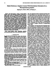
Scenario I: In the first experience, an APPC is run in nominal process in which the buffer flow rate is a nonzero constant value. After finishing the set-point profile, disturbance sequence is applied to the plant in pH=7. Then, the proposed algorithm will control the process. The results are given in tables 3 and 4, and Figs. 2 and 3. Comparisons are based on mean square errors (MSE) between the value of pH and reference model output. Scenario II: First, the process is run by the proposed algorithm in nominal case without disturbance, then in disturbed case, in which there is no buffer, for regulation at given set-point profile. Time duration of each value of setpoint is 4000 samples, which is more than the required time for convergence of the adaptive models. Afterwards, the performance of the closed-loop system is assessed by repeating the test with time duration of 1500 samples. Table 4 collects the results. Discussion: Tables 1 and 2 uncover that time constant and steady-state gain of the process vary with factor of 2 and 150, respectively, in two possible considered cases. Table 3 reveals that by developing a model bank as a memory, the aim of improving the performance of a conventional adaptive controller with a single adaptive model is reached, especially for large variations in set-point. Moreover, according to table 4, disturbance rejection of the proposed algorithm is better than that of APPC. For the first scenario, learning method decided to add 2 models for the first part of the test, i.e. regulation in nominal plant, and it added another model when the buffer stream is cut off in disturbance rejection part; therefore, a model corresponds to the local model in pH=7 without buffer is created. In the second scenario, the objective is to depict the ability of the learning method to add precise local models in a limited number, and in order to improve modelling. On the other hand, the learning method does not intend to add excessive models. As seen in table 5, models that are not selected as the best fixed model for a specific time, and do not help to increase the accuracy of the bank are discarded automatically. Fig. 4 shows that performance index of a fixed model cannot decrease from a specific value, but for an adaptive model the index decreases. Moreover, smaller value for forgetting factor leads to faster decrease in the index, which is beneficial for learning. 6. CONCLUSION In this paper, the problem of improving the performance of a traditional adaptive controller is considered in which a memory is added to the control strategy to keep previous experiences, and finally it ends in a modified approach of multiple models, switching and tuning with the ability of learning of unpredicted situations. The experiences in the form of local models of different operating modes are saved in the model bank. The control signal is designed based on pole-placement control method. The presence of a reinitializable adaptive model which can be converted to a free-running adaptive model assures the stability of closed-

loop system in the linear case. The proposed learning method does not affect stability assurance because stability and performance problems are not related to each other in MMST control strategy. The learning method is designed such that a decision that a new model should be added to the bank is taken whenever the free-running adaptive model gives a model with the sufficient accuracy to describe the current conditions, and the current operating condition differs from those visited a priori; that is, the available fixed model bank has weakness in a sense. In addition, the method is appropriate for modelling of nonlinear plants with local linear models. Some considerations are proposed to enhance the learning algorithm, which makes the algorithm more precise to enlarge the bank without imposing attainable excessive computational complexity. The suggested algorithm is evaluated in a simulated pH neutralization process. The simulation results account that online construction of a local fixed model bank with a desired precision and a limited number of members is advantageous to improve transient response and disturbance rejection. REFERENCES Anderson, B.D.O., Brinsmead, T.S., Bruyne, F.De , Hespanha, J., Liberzon, D. ,and Morse, A.S., (2000). Multiple model adaptive control. Part 1: Finite controller coverings. International Journal of Robust and Nonlinear Control, vol. 10, pp. 909-929. Astrom, K.J., and Wittenmark, B., (1995). Adaptive Control, 2nd ed, Addison-Welsey, NY. Fatehi, A., and Abe, K., (2001). Self-organizing map neural network as a multiple model identifier for time-varying systems. Proceedings of the Sixth International Symposium on Artificial Life and Robotics (AROB 6th ’01), Tokyo, Japan. Filev, D.Sr., and Larsson, T., (2001). Intelligent adaptive control using multiple models. In proceedings of the IEEE international conference on intelligent control, Mexico City, Mexico. Fujinaka, T., and Omatu, S., (1999). A switching scheme for adaptive control using multiple models. In proceedings of the IEEE international conference on systems, man, and cybernetics, Tokyo, Japan. Gundala, R., Hoo, K.A., and Piovoso, M.J., (2000). Multiple model adaptive control design for a MIMO chemical reactor. Ind. Eng. Chem. Res., vol. 39, No. 6, pp.15541564. Henson, R. C. and D. E. Seborg (1994). Adaptive nonlinear control of a pH neutralization process. IEEE Trans. Control Systems Technology, 2, 169-182.

Karimi, A., and Landau, I.D., (2000). Robust adaptive control of a flexible transmission system using multiple models. IEEE Tans. on Control Systems Technology, vol. 8, pp. 321-331. Li, X.R., and Bar-Shalom, Y., (1996). Multiple-model estimation with variable structure. IEEE Transactions on Automatic Control, vol. 41, No. 4, pp. 478-493. Li, X.R., Zhao, Z. and Li, X. B., (2005). General model-set design methods for multiple-model approach. IEEE Transactions on Automatic Control, vol. 50, No. 9, pp.1260–1276. Lourenço, J.M.A., and Lemos, J.M., (2006). Learning in switching multiple model adaptive control. IEEE instrumentation & measurement Magazine, Vol. 9, No. 3, pp. 24-29. Lourenço, J.M.A., and Lemos, J.M., (2007). On-line model bank enlargement for multiple model adaptive control. In proceedings of the European control conference, Kos, Greece. Narendra, K.S. and Balakrishnan J., (1997). Adaptive control using multiple models. IEEE Transactions on Automatic Control, Vol.42, No. 2, pp. 171-187. Narendra, K.S., and Xiang, C., (2000). Adaptive control of discrete-time systems using multiple models. IEEE Trans. on Automatic Control, vol. 45, No. 9, pp. 1669-1686. Narendra, K.S., Balakrishnan, J., and Ciliz, M., (1995). Adaptation and learning using multiple models, switching and tuning. IEEE Control System. Mag., pp. 37–51. Narendra, K.S., Driollet, O.A., Feiler, M. & George, K., (2003). Adaptive control using multiple models, switching and tuning. Int. J. of Adaptive Control and Signal Processing, vol. 14, No 2, pp. 87-102. Narendra, K.S. and Balakrishnan J., (1994). Improving transient response of adaptive control systems using multiple models and switching. IEEE Tans. on Automatic Control, vol. 39, No 9, pp. 1861 -1866. Nelles, O., (2001). Nonlinear system identification. Springer. Petridis, V., and Kehagias, A., (1998). Identification of switching dynamical systems using multiple models. In proceedings of the 37th IEEE conference on Decision and control, Florida, USA, 1998. Pishvaie, M.R., and Shahrokhi, M., (2000). pH control using the nonlinear multiple models, switching, and tuning approach. Ind.. Eng. Chem. Res. vol. 39, No. 5, pp. 13111319. Peymani, E., Fatehi, A., Khaki-Sedigh, A., (2008) A disturbance rejection supervisor in multiple-model based control, proc. of International conference on control, IET, Manchester, UK. Rugh, W.J., and Shamma, J.S., (2000). Research on gain scheduling, survey paper, Automatica, vol. 36, pp.14011425.

Table 1. Parameters of local FOPDT models for the plant in two cases with assumption of constant delay G ( z ) = bz −3 ( z + a)

pH= Nominal case Disturbed case

b a b a

5 0.0143 -0.9895 0.0265 -0.9928

6 0.0032 -0.9910 0.0452 -0.9929

7 0.0037 -0.9927 0.0707 -0.9929

8 0.0178 -0.9931 0.1643 -0.9930

9 0.0069 -0.9933 0.0241 -0.9930

10 0.0009 -0.9942 0.0022 -0.9934

Table 2. Parameters of local FOPDT models for the plant in the case of disturbance sequence with assumption of constant delay around pH=7, G ( z ) = bz −3 ( z + a) Disturbance No.

b a

pH = 7

#1

#2

#3

#4

#5

#6

0.0025 -0.9894

0.0021 -0.9925

0.0009 -0.9938

0.0707 -0.9929

0.0125 -0.9756

0.0026 -0.9947

Table 3. Results of scenario I – MSE of difference between plant and desired output for regulation Range of changes in set-point value APPC MMST with Learning

Table 4. Results of scenario I – MSE of difference between plant and pH =7 for disturbance rejection

Small

Medium

Large

0.6673

0.1077

3.3541

Overall profile 1.3178

0.0117

0.1079

0.6204

0.2154

The worst case Max. Deviation from pH=7 3.01 3.00

APPC MMST+Learning

Overall MSE

MSE

2088 1306

2175 1565

Table 5. Results of scenario II – Learning algorithm, Parameters of created models, when they are created, and final status of them Model No.

b a

Model Parameters Sample of creation Status Set-point value Plant condition

1 0.0144 -0.9894 1691 saved 5

2 0.0033 -0.9908 5037 saved 6

3 0.0267 -0.9927 98502 saved 5

Nominal case – stage 1

4 0.0453 -0.9928 100783 saved 6

5 0.0708 -0.9929 104870 saved 7

6 0.0241 -0.9930 116007 deleted 5

Disturbed case - stage 1

Disturbance Rejection

Identifiation Performance Index

-15

10

x 10

APPC MMST+Learning

7 0.0022 -0.9949 249007 deleted 5 Disturbed case – stage 2

8

Fixed model index re-initializable adap. model index

9.5

6 9

4 2

8

0

pH

8.5

2

7.5

3

4 Time (sec)

5

6

7

7 4

x 10

-20

x 10

free-running adap. model index re-initializable adap. model index

8

6.5 6.94

6.96

6.98

7 Time (sec)

7.02

7.04 5

x 10

Fig. 2. The worst case in comparison of disturbance rejection of MMST with Learning and conventional pole-placement controller.

6 4 2 0 3

3.05

3.1

3.15 Time (sec)

3.2

3.25

3.3 4

x 10

Regulation

Fig. 4. Top: performance index of a fixed model and the reinitializable adaptive model (dashed) at the instant of creating a model. For the fixed model its mean value is a constant, but it decreases for the adaptive one. Bottom: performance index of the free-running adaptive model (dashed) with forgetting factor 0.96 and the reinitializable adaptive model with forgetting factor 0.995. The smaller forgetting value, the faster decrease in the index.

10 9.5 9 8.5

pH

8 7.5 7 6.5 6 APPC MMST+Learning

5.5 5 4.1

4.2

4.3

4.4

4.5 4.6 Time (sec)

4.7

4.8

4.9

5

5.1 5

x 10

Fig. 3. Conventional adaptive pole-placement controller (dashed) vs. MMST with Learning as an Enhanced APPC.