AUTOMATED SUPER-RESOLUTION DETECTION OF FLUORESCENT RODS IN 2D Bo Zhang, Jost Enninga(*), Jean-Christophe Olivo-Marin, Christophe Zimmer Quantitative Image Analysis Group and (*) Unit´e de Pathog´enie Microbienne Mol´eculaire Institut Pasteur, 25 rue du Docteur Roux, 75015 Paris, France ABSTRACT We describe a method designed to detect fluorescent rods from 2D microscopy images. It is motivated by the desire to study the dynamics of bacteria such as Shigella. The methodology is adapted from a super-resolution spot detection algorithm [1] and is based on a parametric model of the rods and the microscope PSF. The algorithm consists of two parts: 1) a pre-detection step, based on thresholding a score computed from the product of the mean curvature and the local intensity of the filtered image, 2) an iterative procedure, where a mixture model of blurred segments is fitted to the image, and segments are removed, then added under the control of hypothesis tests. An upper bound is provided for the probability of erroneously detecting rods in noise. We show that the algorithm can reliably detect and accurately localize rods from low SNR images and can distinguish rods separated by subresolution distances. We also illustrate its ability to identify and separate overlapping bacteria on a real image. 1. INTRODUCTION This paper describes a fully automated method designed to detect thin fluorescent rods. The main applicative goal is to study rod-shaped bacteria, such as Shigella flexneri. In order to understand how these parasites interact with host cells, it is of great interest to localize them and measure their fluorescence intensity over time [2]. Although new insights can be gained by detailed manual analysis of relatively small samples, automated processing of large numbers of images should vastly enrich the study of these dynamic processes. In contrast to highly plastic cells such as amoeba, which call for flexible detection approaches such as deformable models, rod-shaped bacteria have highly constrained shapes, offering the opportunity to use strong shape priors to design more powerful detection techniques, especially for images with low signal-to-noise ratios (SNR). Combined with a model of the microscope point-spread-function (PSF), such methods can also achieve deconvolution and resolve objects below the classical (Rayleigh) resolution limit. The rod detection method presented here is directly inspired by the work of [1] on super-resolution detection of Work funded by Institut Pasteur. E-mail: {bzhang,czimmer}@pasteur.fr
submicrometric fluorescent tags. These tags were modeled as point-like sources, and the PSF as a gaussian, yielding an image model consisting of a mixture of gaussians. In a first step, spots are pre-detected based on a ‘spottiness’ score equal to the product of the local average and the gaussian curvature of the image intensity, providing a score image that is then thresholded using an empirical threshold. In a second step, a parametric model-fitting routine refines the positions of spots, and iteratively inserts new gaussians into the model until the fit to the observed image no longer significantly improves. This second part of the algorithm allows to resolve tags with overlapping fluorescence distributions, for inter-tag distances below the Rayleigh resolution limit (super-resolution). Here, we adapt the approach of [1] to images of rods, modeled as thin segments of constant intensity blurred by the microscope PSF. In section 2, we propose a pre-detection method more suited to rods, and a thresholding scheme that controls the number of false detections. In section 3, we extend the object and image model to fluorescent rods and adapt the model-fitting routine to these structures. In section 4 we report experiments on test images and section 5 provides a brief conclusion. 2. PRE-DETECTION OF RODS This section describes the pre-detection scheme, which aims to provide a good initial guess of the number and position of rods in the image. This initial guess will then be improved upon by the model-fitting approach described in section 3. 2.1. A pixel score for rod detection Following [1], we wish to compute a score allowing to discriminate pixels belonging to rods from bright pixels due to noise. To increase the SNR, we first perform a matched filtering by convolution of the image I with a gaussian filter g of variance σg2 that approximates the microscope PSF [1] (see section 3): I˜ = g ? I, where ? denotes convolution. In [1], a ‘spottiness’ score is then computed for each local maximum as the product of the local average intensity M with the ˜ The gaussian curvature κ (determinant of the Hessian of I). gaussian curvature is well adapted to the detection of isotropic spots, but less so for rods, because a point on a segment has
both a large and a small principal curvature, yielding lower values of the product κ. Both for this reason and for its linearity (see section 2.2), we prefer the mean curvature K (trace ˜ and define the score for of the Hessian, i.e. Laplacian of I) local maxima as follows: S(I) := K(I) · M (I) = (4 ? (g ? I)) · ((g ? A) ? I) (1) where 4 is a convolution kernel approximating the Laplacian operator and A is the 3x3 constant averaging matrix. This score was found to be highly discriminating of rods embedded in very noisy images. 2.2. Controlling false pre-detections For detection of rod pixels, we now wish to determine an appropriate threshold for the score image, as in [1]. Here, however, we seek a threshold that allows to control the false detections. To do this, we need to know the statistical distribution of scores. This is now facilitated by the fact that both K and M are linear operators. In the global null hypothesis H0∗ : {I is gaussian white noise}, K and M are two correlated normal variables. We found that the score S is asymptotically normally (AN ) distributed as stated in Prop. 2.1. Proposition 2.1 If X = (Xi )i∈Zd are i.i.d. normal variables where Xi ∼ N (µ, σ 2 ), then we have: S(X) ∼ AN (µS , σS2 ), µ → ∞, where as σkHk 2 µS σS2
= σ 2 = σ 2 µ2 kLk22 + σ 4 (2 +kHk22 kLk22 )
where d is the image dimension, L = 4 ? g is the Laplacian of Gaussian filter, H = g?A, <·, ·> denotes the inner product and k·k2 is the l2 (Zd )-norm. Prop. 2.1 can be proven using the results on the product of two normal variables [3]. In our case, kHk2 is small (∼10−1 ) and the background intensity µ is high (∼102 ), thus the assumption of Prop. 2.1 is verified even for low SNR. In order to evaluate the two parameters of the normal distribution, we require the image background µ and the gaussian noise variance σ 2 . Here, we automatically estimate µ ˆ from the median of I and σ ˆ from the median absolute deviation estimation of the Daubechies D8 wavelet coefficients at the 1st scale. Now that the distribution of S is known under H0∗ , we can determine a pair of thresholds (tl , tr ) such that the average number of false detections (NFD) over the whole image is lower than a user-defined number FD , e.g. FD = 1. The detected pixels are then simply defined as those for which S 6∈ [tl , tr ]. Since the computation of S is restricted to the ˜ the NFD is strictly bounded by FD . local maxima of I, To each of N0 detected pixels (xi,0 , yi,0 )i=1..N0 , we associate an orientation angle θi,0 computed from the eigenvector of the Hessian corresponding to the lowest eigenvalue, an amplitude Ai,0 = M (xi,0 , yi,0 ) − µ ˆ and an assumed length
Li,0 = L0 . The output of the pre-detection step is thus given by the 5N0 parameters Bi = (xc,i , yc,i , L0 , θi , Ai ), i = 1..N0 , to which we add the estimated background, b0 = µ ˆ. 3. ROD MIXTURE MODEL FITTING The segment parameters computed at this stage are a first guess, which must be improved upon for several reasons. The model-free and local pre-detection scheme described above often produces more than one detection hit for each rod. Conversely, if two or more segments are very close to each other or overlap, the pre-detection may often produce only one hit. Moreover, the localization precision of the pre-detection is limited by the size of the pixels. We therefore seek to improve the pre-detection using a parametric model estimation procedure. This second step aims to: (i) remove redundant segments, (ii) resolve multiple segments that produced a single predetection hit because of overlapping intensities, possibly with super-resolution, (iii) remove residual false detections (pre-detected segments where no segment exists), and (iv) achieve subpixel localization. 3.1. Parametric object and image models In [1], the fluorescent tags are modeled as a finite number of discrete points, uniquely characterized by their 3 spatial coordinates (x, y, z) and their intensity A. Here, we adapt the object model to fluorescent segments of vanishing width. This assumption is valid as long as the transverse dimension of the rod-like object is small relative to the PSF width. In addition, we assume that the intensity is constant along the rod. Each rod is then uniquely characterized by only 5 parameters: B = (xc , yc , θ, L, A), where (xc , yc ) are the coordinates of the segment center, θ is its angle with the x-axis, L = 2l the segment length, and A its peak intensity. In this paper, we will also assume that the rod has a known length of L0 , reducing the number of free parameters to 4. The contribution of a fluorescent segment B to the image at location (x, y) can then be written: Z
1
g (x − x(t), y − y(t)) ldt
IB (x, y) = A
(2)
−1
where x(t) = xc + tl cos(θ), y(t) = yc + tl sin(θ) and g is the microscope PSF.�As in [1],�we use a gaussian approxima2 +y 2 . Analytical expressions of σg tion: g(x, y) = exp − x 2σ 2 g as function of microscopy parameters are given for widefield microscopy in [1] and were recently worked out for widefield, laser and disk scanning confocal microscopes in [4, 5]. Combining the previous equations, we obtain: � � cos θ)2 IB (x, y) = AG exp − (X sin θ−Y · 2 2σg h � � � �i √ θ−Y sin θ + erf l+X cos √ θ+Y sin θ erf l−X cos (3) 2σ 2σ g
g
where X = x−x R x c , Y2 = y−yc , erf denotes the error function: erf(x) = √2π 0 e−t dt, and G is a normalization factor such that the peak intensity IB (xc , yc ) = A. Images containing several rods are now modeled as a superposition of the intensity distributions of N individual rods Bi = (xc,i , yc,i , L0 , θi , Ai ), i = 1..N and a uniform background b. The full image model is thus: MN (x, y) = b + ΣN i=1 IBi (x, y)
(4)
This top-down procedure removes redundant segments, but we also wish to distinguish overlapping or closely spaced rod objects. For such cases, the pre-detection may in fact underestimate the number of segments. For this reason, we follow up with a bottom-up addition of segments, where the hypothesis test described above is applied in reverse, i.e. as in [1] : segments are added to the model as long as they significantly increase the quality of the fit. The program stops when the fit can no longer be improved by adding new segments, and outputs the rod parameters from the final fit.
3.2. Iterative model fitting and hypothesis tests We now describe how the mixture model (4) is used and how the rod parameters are estimated, starting from the initial guess provided by the pre-detection step. The two ingredients employed here are a fit of the model to the image, and a hypothesis testing scheme that controls how the number of segments in the model is changed [1]. For a given number of rods N , the fit is performed by gradient descent minimization of the mean square difference RN between the model MN and the Ny 2 x image I: RN (P ) = ΣN i=1 Σj=1 (MN (i, j) − I(i, j)) , where Nx and Ny are the number of image columns and rows. At the onset, the model fitting is initialized with the parameter P = (N0 , b0 , {Bi,0 = (xi,0 , yi,0 , θi,0 , L0 , Ai,0 )}i=1..N0 ) of the predetection of section 2. The initial fit of MN0 produces a refined estimation of the rod parameters Bi allowing subpixelic localization. At this stage, however, redundant segments are generally present in the model, since actual rods in the image often give rise to several pre-detections, as mentioned earlier. Superfluous segments may also be present in the image background due to residual false positives of the pre-detection. We therefore seek to remove segments that are not necessary to model the image. To do this we sequentially try to remove segments from the model using hypothesis tests to decide whether to accept segment removal or not. This top-down approach is a reversal of the bottom-up method of [1], where the number of spots is only allowed to increase. After removing a segment from model MN , we fit the new model MN −1 to the image, and then ask whether the new fit is significantly worse than the previous fit. This is done by testing the null hypothesis H0 : s2N −1 = s2N against the alternative H1 : s2N −1 > s2N . Here, s2N = RN /rN and RN /σ 2 is the χ2 statistics with rN = Nx Ny − pN degrees of freedom, where pN = 4N + 1 is the number of free parameters of the model MN . We res2
ject H0 if the test statistics T = Ns2−1 exceeds the threshold N T0 determined from the Fisher distribution and the confidence level α (we used α = 0.05). If H0 is maintained (T ≤ T0 ), we remove the segment from the model, since the smaller model MN −1 provides an equally good fit to the data as MN ; otherwise, the removed segment is put back into the model, and another segment is examined. This procedure is repeated until no segment can be removed without significantly degrading the fit.
3.3. Controlling false detections Thanks to the hypothesis tests used in sections 2.2 and 3.2, we can control the false rod detections at the end of the algorithm. Assuming that the decisions to remove segments in the top-down procedure are independent, the probability bound of falsely detecting n > 0 rods in a large rod-free image is: lim
Nx ·Ny →∞
Pr(n > 0|H0∗ ) ≤ 1 − e−Fp α
4. EXPERIMENTS To quantitatively evaluate the performance of the algorithm, we run series of experiments on simulated data. Noise-free images were simulated using the model of section 3.1 and the following parameters: pixel sizes 0.05×0.05µm, L0 = 2µm, A = 1, Nx = Ny = 100 and σg = 0.1µm, a value appropriate for a disk scanning confocal microscope with typical microscopy settings [5]. Additive gaussian noise of mean 2 was then added to produce images µ = 90 and variance σN at various SNR, defined here as SNR= A/σN . 0
0
0
0
0
0.5
0.5
0.5
0.5
0.5
1
1
1
1
1
1.5
1.5
1.5
1.5
1.5
2
2
2
2
2
2.5
2.5
2.5
2.5
2.5
3
3
3
3
3
3.5
3.5
3.5
3.5
3.5
4
4
4
4
4
4.5
4.5
4.5
4.5
4.5
5
0
0.5
1
1.5
2
2.5
3
3.5
4
4.5
5
5
0
0.5
1
1.5
2
2.5
3
3.5
4
4.5
5
5
0
0.5
1
1.5
2
2.5
3
3.5
4
4.5
5
5
0
0.5
1
1.5
2
2.5
3
3.5
4
4.5
5
5
0
0.5
1
1.5
2
2.5
3
3.5
4
4.5
5
Fig. 1. Simulated test images of an isolated rod for SNR= 1, 2, 3, 4 and 5 (from left to right). Image size: 5µm × 5µm.
SNR
CDR (%)
RMSE(x,y) (nm)
RMSEθ (deg.)
RMSEA
1 2 2.5 3 4 5 10 50
0 95 100 100 100 100 100 100
19.8 18.9 13.4 9.9 5.0 1.0
0.50 0.38 0.31 0.25 0.10 0.027
0.033 0.029 0.022 0.017 0.010 0.0018
Table 1. Detection performance as function of SNR. Based on 100 simulated images for each SNR. CDR= correct detection rate; RMSE=root mean square error. The 3 columns on the right show the RMSE of position, orientation and amplitude.
4.1. Detecting isolated rods We first test our algorithm on images of a single rod, without the complications due to overlapping fluorescence from several rods. Example images are shown in Fig.1 and numeric results are given in Table 1. Based on these trials, we find that the algorithm reliably detects exactly 1 segment for SNR as low as 2.5, underlining the robustness of the algorithm to noise. Detection becomes unreliable for SNR=2, and completely breaks down for SNR=1. Table 1 also indicates the errors made in estimating rod parameters for SNR≥2.5. Similarly to spot detection [1], the localization errors are in the range of tens of nanometers only for even the lowest detectable SNR. The orientation is estimated with an error < 1 deg. The accuracy of rod intensity estimation is also very high, with errors of a few percent only. 4.2. Separating close or overlapping rods In order to test the ability of the algorithm to separate segments whose fluorescence overlap (Fig. 2), we now simulate images of two parallel segments for various inter-segment distances d and SNR. We find that the rods can be resolved at distances well below the approximate Rayleigh resolution limit of two parallel lines dR ≈ 280nm for SNR as low as 4 (see Table 2). A super-resolution factor of 2 is reached for SNR between 5 and 10. 0
0
0.5
0.5
1
1
1.5
1.5
2
2
2.5
2.5
3
3
3.5
3.5
4
4
4.5
5
4.5
0
0.5
1
1.5
2
2.5
3
3.5
4
4.5
5
5
0
0.5
1
1.5
2
2.5
3
3.5
4
4.5
5
Fig. 2. Super-resolution detection of two parallel rods separated by d = 0.2µm < dR . The two fluorescence distributions merge, but the algorithm nevertheless resolves the two segments. Left: simulated image with SNR=5. Right: simulated noise-free image with the 2 detected segments shown in green.
SNR 2 3 4 5 10
d = 100 0 0 0 0 80
d = 150 0 0 0 70 100
d = 200 < dR ≈ 280 0 70 100 100 100
d = 500 100 100 100 100 100
Table 2. Resolution performance as function of SNR and distance
is not strictly valid. We chose to address this here by artificially adjusting σg to 0.18µm. Despite the imperfection of the model, it is apparent from Fig. 3 that the algorithm successfully detects overlapping bacteria. model image 0
0
1
1
2
2
3
3
4
4
5
5
6
6
0
1
2
3
4
5
6
0
1
2
3
4
5
6
Fig. 3. Detecting overlapping bacteria in a real image. Left: original image, obtained from a z-sum of a 3D stack acquired with a disk scanning confocal microscope. Middle: with detected rods (green segments); red segments indicate the result of pre-detection. Note that the pre-detection alone cannot resolve the two overlapping bacteria. Right: model image M computed from the detection result.
5. CONCLUSION We have described our first version of a fully automated method for detection of fluorescent segments. The experiments show that the method is specially suited to localize and quantify the fluorescence of these objects in low SNR images and that it can distinguish overlapping segments with super-resolution. Encouraging first results are obtained in detecting fluorescently labeled bacteria. We plan to pursue this work along several lines, including extension to 3D data, images with both Poisson and gaussian noise, inclusion of a tracking scheme for time sequence analysis, and extension to tubes of finite width. 6. REFERENCES [1] D. Thomann, D. R. Rines, P. K. Sorger, and G. Danuser, “Automatic fluorescent tag detection in 3D with super-resolution: application to the analysis of chromosome movement,” J. Microsc., vol. 208, pp. 49–64, October 2002. [2] J. Enninga, J. Mounier, P. Sansonetti, and G. Tran Van Nhieu, “Studying the Secretion of Type III Effectors into Host Cells in Real Time,” Nature Methods, vol. 2, no. 12, pp. 959–965, 2005. [3] L. A. Aroian, “The Probability Function of the Product of Two Normally Distributed Variables,” Ann. Math. Statist., vol. 18, pp. 265–271, 1947.
between segments (d in nm). Entries are the CDR based on 10 trials each (in %).
[4] B. Zhang, J. Zerubia, and J.-C. Olivo-Marin, “A study of Gaussian approximations of fluorescence microscopy PSF models,” in Three-dim. and multidim. micr.: Image acquis. and proc. XIII, 2006, vol. 6090 of Proc. SPIE, in press.
4.3. Illustration on real data
[5] B. Zhang and J.-C. Olivo-Marin, “Gaussian Approximations of Laser/Disk Scanning Confocal Microscopy PSF Models,” Tech. Rep., Institut Pasteur, 2005.
Finally, Fig.3 shows an example of a real image of fluorescently labeled Shigella flexneri [2]. Because these bacteria have diameters of ∼ 0.4µm, the zero width segment model