1 Auditory Sparse Coding Steven R. Ness University of Victoria Thomas Walters Google Inc. Richard F. Lyon Google Inc.

CONTENTS 1.1 1.2 1.3

1.4 1.5

1.1

Summary . . . . . . . . . . . . . . . . . . . . . . . . . . . . . . . . . . . . . . . . . . . . . . . . . . . . . . . . . . . . . . . . . . Introduction . . . . . . . . . . . . . . . . . . . . . . . . . . . . . . . . . . . . . . . . . . . . . . . . . . . . . . . . . . . . . . . 1.2.1 The stabilized auditory image . . . . . . . . . . . . . . . . . . . . . . . . . . . . . . . . . . . . Algorithm . . . . . . . . . . . . . . . . . . . . . . . . . . . . . . . . . . . . . . . . . . . . . . . . . . . . . . . . . . . . . . . . . 1.3.1 Pole–Zero Filter Cascade . . . . . . . . . . . . . . . . . . . . . . . . . . . . . . . . . . . . . . . . . . 1.3.2 Image Stabilization . . . . . . . . . . . . . . . . . . . . . . . . . . . . . . . . . . . . . . . . . . . . . . . . 1.3.3 Box Cutting . . . . . . . . . . . . . . . . . . . . . . . . . . . . . . . . . . . . . . . . . . . . . . . . . . . . . . . 1.3.4 Vector Quantization . . . . . . . . . . . . . . . . . . . . . . . . . . . . . . . . . . . . . . . . . . . . . . . 1.3.5 Machine Learning . . . . . . . . . . . . . . . . . . . . . . . . . . . . . . . . . . . . . . . . . . . . . . . . . Experiments . . . . . . . . . . . . . . . . . . . . . . . . . . . . . . . . . . . . . . . . . . . . . . . . . . . . . . . . . . . . . . . 1.4.1 Sound Ranking . . . . . . . . . . . . . . . . . . . . . . . . . . . . . . . . . . . . . . . . . . . . . . . . . . . . 1.4.2 MIREX 2010 . . . . . . . . . . . . . . . . . . . . . . . . . . . . . . . . . . . . . . . . . . . . . . . . . . . . . . Conclusions . . . . . . . . . . . . . . . . . . . . . . . . . . . . . . . . . . . . . . . . . . . . . . . . . . . . . . . . . . . . . . . .

3 4 6 7 7 8 9 9 10 11 11 14 17

Summary

The concept of sparsity has attracted considerable interest in the field of machine learning in the past few years. Sparse feature vectors contain mostly values of zero and one or a few non-zero values. Although these feature vectors can be classified by traditional machine learning algorithms, such as SVM, there are various recently-developed algorithms that explicitly take advantage of the sparse nature of the data, leading to massive speedups in time, as well as improved performance. Some fields that have benefited from the use of sparse algorithms are finance, bioinformatics, text mining [1], and image classification [4]. Because of their speed, these algorithms perform well on very large collections of data [2]; large collections are becoming increasingly 3

4

Book title goes here

relevant given the huge amounts of data collected and warehoused by Internet businesses. In this chapter, we discuss the application of sparse feature vectors in the field of audio analysis, and specifically their use in conjunction with preprocessing systems that model the human auditory system. We present early results that demonstrate the applicability of the combination of auditory-based processing and sparse coding to content-based audio analysis tasks. We present results from two different experiments: a search task in which ranked lists of sound effects are retrieved from text queries, and a music information retrieval (MIR) task dealing with the classification of music into genres.

1.2

Introduction

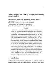
Traditional approaches to audio analysis problems typically employ a shortwindow fast Fourier transform (FFT) as the first stage of the processing pipeline. In such systems a short, perhaps 25ms, segment of audio is taken from the input signal and windowed in some way, then the FFT of that segment is taken. The window is then shifted a little, by perhaps 10ms, and the process is repeated. This technique yields a two-dimensional spectrogram of the original audio, with the frequency axis of the FFT as one dimension, and time (quantized by the step-size of the window) as the other dimension. While the spectrogram is easy to compute, and a standard engineering tool, it bears little resemblance to the early stages of the processing pipeline in the human auditory system. The mammalian cochlea can be viewed as a bank of tuned filters the output of which is a set of band-pass filtered versions of the input signal that are continuous in time. Because of this property, fine-timing information is preserved in the output of cochlea, whereas in the spectrogram described above, there is no fine-timing information available below the 10ms hop-size of the windowing function. This fine-timing information from the cochlea can be made use of in later stages of processing to yield a three-dimensional representation of audio, the stabilized auditory image (SAI)[11], which is a movie-like representation of sound which has a dimension of ‘time-interval’ in addition to the standard dimensions of time and frequency in the spectrogram. The periodicity of the waveform gives rise to a vertical banding structure in this time interval dimension, which provides information about the sound which is complementary to that available in the frequency dimension. A single example frame of a stabilized auditory image is shown in Figure 1.1. While we believe that such a representation should be useful for audio analysis tasks, it does come at a cost. The data rate of the SAI is many times that of the original input audio, and as such some form of dimensionality

Auditory Sparse Coding

5

reduction is required in order to create features at a suitable data rate for use in a recognition system. One approach to this problem is to move from a the dense representation of the SAI to a sparse representation, in which the overall dimensionality of the features is high, but only a limit number of the dimensions are nonzero at any time. In recent years, machine learning algorithms that utilize the properties of sparsity have begun to attract more attention and have been shown to outperform approaches that use dense feature vectors. One such algorithm is the passive-aggressive model for image retrieval (PAMIR), a machine learning algorithm that learns a ranking function from the input data, that is, it takes an input set of documents and orders them based on their relevance to a query. PAMIR was originally developed as a machine vision method and has demonstrated excellent results in this field. There is also growing evidence that in the human nervous system sensory inputs are coded in a sparse manner; that is, only small numbers of neurons are active at a given time [10]. Therefore, when modeling the human auditory system, it may be advantageous to investigate this property of sparseness in relation to the mappings that are being developed. The nervous systems of animals have evolved over millions of years to be highly efficient in terms of energy consumption and computation. Looking into the way sound signals are handled by the auditory system could give us insights into how to make our algorithms more efficient and better model the human auditory system. One advantage of using sparse vectors is that such coding allows very fast computation of similarity, with a trainable similarity measure [4]. The efficiency results from storing, accessing, and doing arithmetic operations on only the non-zero elements of the vectors. In one study that examined the performance of sparse representations in the field of natural language processing, a 20- to 80-fold speedup over LIBSVM was found [7]. They comment that kernel-based methods, like SVM, scale quadratically with the number of training examples and discuss how sparsity can allow algorithms to scale linearly based on the number of training examples. In this chapter, we use the stabilized auditory image (SAI) as the basis of a sparse feature representation which is then tested in a sound ranking task and a music information retrieval task. In the sound raking task, we generate a two-dimensional SAI for each time slice, and then sparse-code those images as input to PAMIR. We use the ability of PAMIR to learn representations of sparse data in order to learn a model which maps text terms to audio features. This PAMIR model can then be used rank a list of unlabeled sound effects according to their relevance to some text query. We present results that show that in certain tasks our methods can outperform highly tuned FFT based approaches. We also use similar sparse-coded SAI features as input to a music genre classification system. This system uses an SVM classifier on the sparse features, and learns text terms associated with music. The system was entered into the annual music information retrieval evaluation exchange evaluation (MIREX 2010).

6

Book title goes here

Results from the sound-effects ranking task show that sparse auditorymodel-based features outperform standard MFCC features, reaching precision about 73% for the top-ranked sound, compared to about 60% for standard MFCC and 67% for the best MFCC variant. These experiments involved ranking sounds in response to text queries through a scalable online machine learning approach to ranking.

1.2.1

The stabilized auditory image

In our system we have taken inspiration from the human auditory system in order to come up with a rich set of audio features that are intended to more closely model the audio features that we use to listen and process music. Such fine timing relations are discarded by traditional spectral techniques. A motivation for using auditory models is that the auditory system is very effective at identifying many sounds. This capability may be partially attributed to acoustic features that are extracted at the early stages of auditory processing. We feel that there is a need to develop a representation of sounds that captures the full range of auditory features that humans use to discriminate and identify different sounds, so that machines have a chance to do so as well.

FIGURE 1.1 An example of a single SAI of a sound file of a spoken vowel sound. The vertical axis is frequency with lower frequencies at the bottom of the figure and higher frequencies on the top. The horizontal axis is the autocorrelation lag. From the positions of the vertical features, one can determine the pitch of the sound. This SAI representation generates a 2D image from each section of waveform from an audio file. We then reduce each image in several steps: first cutting the image into overlapping boxes converted to fixed resolution per box; second, finding row and column sums of these boxes and concatenating those into a vector; and finally vector quantizing the resulting medium-

Auditory Sparse Coding

7

dimensionality vector, using a separate codebook for each box position. The VQ codeword index is a representation of a 1-of-N sparse code for each box, and the concatenation of all of those sparse vectors, for all the box positions, makes the sparse code for the SAI image. The resulting sparse code is accumulated across the audio file, and this histogram (count of number of occurrences of each codeword) is then used as input to an SVM [5] classifier[3]. This approach is similar to that of the “bag of words” concept, originally from natural language processing, but used heavily in computer vision applications as “bag of visual words”; here we have a “bag of auditory words”, each “word” being an abstract feature corresponding to a VQ codeword. The bag representation is a list of occurrence counts, usually sparse.

1.3

Algorithm

In our experiments, we generate a stream of SAIs using a series of modules that process an incoming audio stream through the various stages of the auditory model. The first module filters the audio using the pole–zero filter cascade (PZFC) [9], then subsequent modules find strobe points in this audio, and generate a stream of SAIs at a rate of 50 per second. The SAIs are then cut into boxes and are transformed into a high dimensional dense feature vector [12] which is vector quantized to give a high dimensional sparse feature vector. This sparse vector is then used as input to a machine learning system which performs either ranking or classification. This whole process is shown in diagrammatic form in Figure 1.2

1.3.1

Pole–Zero Filter Cascade

We first process the audio with the pole–zero filter cascade (PZFC) [9], a model inspired by the dynamics of the human cochlea. The PZFC is a cascade of a large number of simple filters with an output tap after each stage. The effect of this filter cascade is to transform an incoming audio signal into a set of band-pass filtered versions of the signal. In our case we used a cascade with 95 stages, leading to 95 output channels. Each output channel is halfwave rectified to simulate the output of the inner hair cells along the length of the cochlea. The PZFC also includes an automatic gain control (AGC) system that mimics the effect of the dynamic compression mechanisms seen in the cochlea. A smoothing network, fed from the output of each channel, dynamically modifies the characteristics of the individual filter stages. The AGC can respond to changes in the output on the timescale of milliseconds, leading to very fast-acting compression. One way of viewing this filter cascade is that its outputs are an approximation of the instantaneous neuronal firing rate as a function of cochlear place, modeling both the frequency filtering and

8

Book title goes here

FIGURE 1.2 A flowchart describing the flow of data in our system. First, either the pole– zero filter cascade (PZFC) or gammatone filterbank filters the input audio signal. Filtered signals then pass through a half-wave rectification module (HCL), and trigger points in the signal are then calculated by the local-max module. The output of this stage is the SAI, the image in which each signal is shifted to align the trigger time to the zero lag point in the image. The SAI is then cut into boxes with the box-cutting module, and the resulting boxes are then turned into a codebook with the vector-quantization module. the automatic gain control characteristics of the human cochlea [8]. The PZFC parameters used for the sound-effects ranking task are described in [9]. We did not do any further tuning of this system to the problems of genre, mood or song classification; this would be a fruitful area of further research.

1.3.2

Image Stabilization

The output of the PZFC filterbank is then subjected to a process of strobe finding where large peaks in the PZFC signal are found. The temporal locations of these peaks are then used to initiate a process of temporal integration whereby the stabilized auditory image is generated. These strobe points “stabilize” the signal in a manner analogous to the trigger mechanism in an oscilloscope. When these strobe points are found, a modified form of autocorrelation, known as strobed temporal integration, which is like a sparse version of autocorrelation where only the strobe points are correlated against the sig-

Auditory Sparse Coding

9

FIGURE 1.3 The cochlear model, a filter cascade with half-wave rectifiers at the output taps, and an automatic gain control (AGC) filter network that controls the tuning and gain parameters in response to the sound. nal. Strobed temporal integration has the advantage of being considerably less computationally expensive than full autocorrelation.

1.3.3

Box Cutting

We then divide each image into a number of overlapping boxes using the same process described in [9]. We start with rectangles of size 16 lags by 32 frequency channels, and cover the SAI with these rectangles, with overlap. Each of these rectangles is added to the set of rectangles to be used for vector quantization. We then successively double the height of the rectangle up to the largest size that fits in an SAI frame, but always reducing the contents of each box back to 16 by 32 values. Each of these doublings is added to the set of rectangles. We then double the width of each rectangle up to the width of the SAI frame and add these rectangles to the SAI frame. The output of this step is a set of 44 overlapping rectangles. The process of box-cutting is shown in Figure 1.4. In order to reduce the dimensionality of these rectangles, we then take their row and column marginals and join them together into a single vector.

1.3.4

Vector Quantization

The resulting dense vectors from all the boxes of a frame are then converted to a sparse representation by vector quantization. We first preprocessed a collection of 1000 music files from 10 genres using a PZFC filterbank followed by strobed temporal integration to yield a set of

10

Book title goes here

FIGURE 1.4 The boxes, or multi-scale regions, used to analyze the stabilized auditory images are generated in a variety of heights, widths, and positions.

SAI frames for each file . We then take this set of SAI and apply the boxcutting technique described above. The followed by the calculation of row and column marginals. These vectors are then used to train dictionaries of 200 entries, representing abstract “auditory words”, for each box position, using a k-means algorithm. This process requires the processing of large amounts of data, just to train the VQ codebooks on a training corpus. The resulting dictionaries for all boxes are then used in the MIREX experiment to convert the dense features from the box cutting step on the test corpus songs into a set of sparse features where each box was represented by a vector of 200 elements with only one element being non-zero. The sparse vectors for each box were then concatenated, and these long spare vectors are histogrammed over the entire audio file to produce a sparse feature vector for each song or sound effect. This operation of constructing a sparse bag of auditory words was done for both the training and testing corpora.

Auditory Sparse Coding

1.3.5

11

Machine Learning

For this system, we used the support vector machine learning system from libSVM which is included in the Marsyas[13] framework. Standard Marsyas SVM parameters were used in order to classify the sparse bag of auditory words representation of each song. It should be noted that SVM is not the ideal algorithm for doing classification on such a sparse representation, and if time permitted, we would have instead used the PAMIR machine learning algorithm as described in [9]. This algorithm has been shown to outperform SVM on ranking tasks, both in terms of execution speed and quality of results.

1.4 1.4.1

Experiments Sound Ranking

We performed an experiment in which we examined a quantitative ranking task over a diverse set of audio files using tags associated with the audio files. For this experiment, we collected a dataset of 8638 sound effects, which came from multiple places. 3855 of the sound files were from commercially available sound effect libraries, of these 1455 were from the BBC sound effects library. The other 4783 audio files were collected from a variety of sources on the internet, including findsounds.com, partnersinrhyme.com, acoustica.com, ilovewaves.com, simplythebest.net, wav-sounds.com, wav-source.com and wavlist.com. We then manually annotated this dataset of sound effects with a small number of tags for each file. Some of the files were already assigned tags and for these, we combined our tags with this previously existing tag information. In addition, we added higher level tags to each file, for example, files with the tags “cat”, “dog” and “monkey” were also given the tags “mammal” and “animal”. We found that the addition of these higher level tags assist retrieval by inducing structure over the label space. All the terms in our database were stemmed, and we used the Porter stemmer for English, which left a total of 3268 unique tags for an average of 3.2 tags per sound file. In order to estimate the performance of the learned ranker, we used a standard three-fold cross-validation experimental setup. In this scheme, two thirds of the data is used for training and one third is used for testing; this process is then repeated for all three splits of the data and results of the three are averaged. We removed any queries that had fewer than 5 documents in either the training set or the test set, and if the corresponding documents had no other tags, these documents were removed as well. To determine the values of the hyperparameters for PAMIR we performed a second level of cross-validation where we iterated over values for the aggressiveness parameter C and the number of training iterations. We found that in

12

Book title goes here

general system performance was good for moderate values of C and that lower values of C required a longer training time. For the agressiveness parameter, we selected a value of C=0.1, a value which was also found to be optimal in other research [6]. For the number of iterations, we chose 10M, and found that in our experience, the system was not very sensitive to the exact value of these parameters. We evaluated our learned model by looking at the precision within the top k audio files from the test set as ranked by each query. Precision at top k is a commonly used measure in retrieval tasks such as these and measures the fraction of positive results within the top k results from a query. The stabilized auditory image generation process has a number of parameters which can be adjusted including the parameters of the PZFC filter and the size of rectangles that the SAI is cut into for subsequent vector quantization. We created a default set of parameters and then varied these parameters in our experiments. The default SAI box-cutting was performed with 16 lags and 32 channels, which gave a total of 49 rectangles. These rectangles were then reduced to their marginal values which gives a 48 dimension vector, and a codebook of size 256 was used for each box, giving a total of 49 x 256 = 12544 feature dimensions. Starting from these, we then made systematic variations to a number of different parameters and measured their effect on precision of retrieval. For the box-cutting step, we adjusted various parameters including the smallest sized rectangle, and the maximum number of rectangles used for segmentation. We also varied the codebook sizes that we used in the sparse coding step. In order to evaluate our method, we compared it with results obtained using a very common feature extraction method for audio analysis, MFCCs (mel-frequency cepstral coefficients). In order to compare this type of feature extraction with our own, we turned these MFCC coefficients into a sparse code. These MFCC coefficients were calculated with a Hamming window with initial parameters based on a setting optimized for speech. We then changed various parameters of the MFCC algorithm, including the number of cepstral coefficients (13 for speech), the length of each frame (25ms for speech), and the number of codebooks that were used to sparsify the dense MFCC features for each frame. We obtained the best performance with 40 cepstral coefficients, a window size of 40ms and codebooks of size 5000. We investigated the effect of various parameters of the SAI feature extraction process on test-set precision, these results are displayed graphically in Figure 1.5 where the precision of the top ranked sound file is plotted against the number of features used. As one can see from this graph, performance saturates when the number of features approaches 105 which results from the use of 4000 code words per codebook, with a total of 49 codebooks. This particular set of parameters led to a performance of 73%, significantly better than the best MFCC result which achieved a performance of 67%, which represents a smaller error of 18% (from 33 % to 27 % error). It is also notable

Auditory Sparse Coding

13

FIGURE 1.5 Ranking at top-1 retrieved result for all the experimental runs described in this section. A few selected experiment names are plotted next to each point, and different experiments are shown by different icons. The convex hull that connects the best-performing experiments is plotted as a solid line. that SAI can achieve better precision-at-top-k consistently for all values of k, albeit with a smaller improvement in relative precision. In table 1.2 results of three queries along with the top five sound files that were returned by the best SAI-based and MFCC-based systems. From this table, one can see that the two systems perform in different ways, this can be expected when one considers the basic audio features that these two systems extract. For example, for the query “gulp”, the SAI system returns “pouring” and “water-dripping”, all three of these share the similarity of involving the movement of water or liquids. When we calculated performance, it was based on textual tags, which are often noisy and incomplete. Due to the nature of human language and perception, people often use different words to describe sounds that are very similar, for example, a Chopin Mazurka could be described with the words “piano”, “soft”, “classical”, “Romantic”, and “mazurka”. To compound this difficulty, a song that had a female vocalist singing could be labelled as “woman”, “women”, “female”, “female vocal”, or “vocal”. This type of multi-label problem is common in the field of content based retrieval. It can be alleviated by a number of techniques, including the stemming of words, but due to the varying nature of human language and perception, will continue to remain an issue. In Figure 1.6 the performance of the SAI and MFCC based systems are

14

Book title goes here

FIGURE 1.6 A comparison of the average precision of the SAI and MFCC based systems. Each point represents a single query, with the horizontal position being the MFCC average precision and the vertical position being the SAI average precision. More of the points appear above the y=x line, which indicates that the SAI based system achieved a higher mean average precision.

compared to each other with respect to their average precision. A few select full tag names are placed on this diagram, for the rest, only a plus is shown. This is required because otherwise the text would overlap to such a great degree that it would be impossible to read. In this diagram we plot the average precision of the SAI based system against that of the MFCC based system, with the SAI precision shown along the vertical axis and the MFCC precision shown along the horizontal axis. If the performance of the two systems was identical, all points would lie on the line y=x. Because more points lie above the line than below the line, the performance of the SAI based system is better than that of the MFCC based system.

Auditory Sparse Coding

top-k 1 2 5 10 20

SAI 27 39 60 72 81

MFCC 33 44 62 74 84

15

percent error reduction 18 % 12 % 4% 3% 4%

TABLE 1.1 A comparison of the best SAI and MFCC configurations. This table shows the percent error at top-k, where error is defined as 1 - precision.

Query tarzan

SAI file (labels) MFCC file (labels) Tarzan-2 (tarzan, yell) TARZAN (tarzan, yell) tarzan2 (tarzan, yell) 175orgs (steam, whistle) 203 (tarzan) mosquito-2 (mosquito) wolf (mammal, wolves, wolf, ...) evil-witch-laugh (witch, evil, laugh) morse (morse, code) Man-Screams (horror, scream, man) applause 27-Applause-from-audience 26-Applause-from-audience audience 30-Applause-from-audience phase1 (trek, phaser, star) golf50 (golf) fanfare2 (fanfare, trumpet) firecracker 45-Crowd-Applause (crowd, applause) 53-ApplauseLargeAudienceSFX golf50 gulp tite-flamn (hit, drum, roll) GULPS (gulp, drink) water-dripping (water, drip) drink (gulp, drink) Monster-growling (horror, monster, growl) california-myotis-search (blip) Pouring (pour,soda) jaguar-1 (bigcat, jaguar, mammal, ...) TABLE 1.2 A comparison of the best SAI and MFCC configurations. This table shows the percent error at top-k, where error is defined as (1 - precision).

16

Book title goes here Algorithm SAI/VQ Marsyas MFCC Best Average

Classification Accuracy 0.4987 0.4430 0.6526 0.455

TABLE 1.3 Classical composer train/test classification task Algorithm SAI/VQ Marsyas MFCC Best Average

Classification Accuracy 0.4861 0.5750 0.6417 0.49

TABLE 1.4 Music mood train/test classification task

1.4.2

MIREX 2010

All of these algorithms were then ported to the Marsyas music information retrieval framework from AIM-C, and extensive tests were written as described above. These algorithms were submitted to the MIREX 2010 competition as C++ code, which was then run by the organizers on blind data. As of this date, only results for two of the four train/test tasks have been released. One of these is for the task of classifying classical composers and the other is for classifying the mood of a piece of music. There were 40 groups participating in this evaluation, the most ever for MIREX, which gives some indication about how this classification task is increasingly important in the real world. Below I present the results for the best entry, the average of all entries, our entry, and the other entry for the Marsyas system. It is instructive to compare our result to that of the standard Marsyas system because in large part we would like to compare the SAI audio feature to the standard MFCC features, and since both of these systems use the SVM classifier, we partially negate the influence of the machine learning part of the problem. For the classical composer task the results are shown in table 1.3 and for the mood classification task, results are shown in table 1.4 From these results we can see that in the classical composer task we outperformed the traditional Marsyas system which has been tuned over the course of a number of years to perform well. This gives us the indication that the use of these SAI features has promise. However, we underperform the best algorithm, which means that there is work to be done in terms of testing different machine learning algorithms that would be better suited to this type of data. However, in a more detailed analysis of the results, which is shown in 1.7, it is evident that each of the algorithms has a wide range of perfor-

Auditory Sparse Coding

17

mance on different classes. This graph shows that the most well predicted in our SAI/VQ classifier overlap significantly with those from the highest scoring classification engines.

FIGURE 1.7 Per class results for classical composer

In the mood task, we underperform both Marsyas and the leading algorithm. This is interesting and might speak to the fact that we did not tune the parameters of this algorithm for the task of music classification, but instead used the parameters that worked best for the classification of sound effects. Music mood might be a feature that has spectral aspects that evolve over longer time periods than other features. For this reason, it would be important to search for other parameters in the SAI algorithm that would perform well for other tasks in music information retrieval. For these results, due to time constraints, we only used the SVM classifier on the SAI histograms. This has been shown in [9] to be an inferior classifier for this type of sparse, high-dimensional data than the PAMIR algorithm. In the future, we would like to add the PAMIR algorithm to Marsyas and to try these experiments using this new classifier. It was observed that the MIR community is increasingly becoming focused on advanced machine learning techniques, and it is clear that it will be critical to both try different machine learning algorithms on these audio features as well as to perform wider sweeps of parameters for these classifiers. Both of these will be important in increasing the performance of these novel audio features.

18

1.5

Book title goes here

Conclusions

The use of physiologically-plausible acoustic models combined with a sparsification approach has shown promising results in both the sound effects ranking and MIREX 2010 experiments. These features are novel and hold great promise in the field of MIR for the classification of music as well as other tasks. Some of the results obtained were better than that of a highly tuned MIR system on blind data. In this task we were able to expose the MIR community to these new audio features. These new audio features have been shown to outperform MFCC features in a sound-effects ranking task, and by evaluating these features with machine learning algorithms more suited for these high dimensional, sparse features, we have great hope that we will obtain even better results in future MIREX evaluations.

Bibliography [1] Suhrid Balakrishnan and David Madigan. Algorithms for sparse linear classifiers in the massive data setting. J. Mach. Learn. Res., 9:313–337, 2008. [2] L´eon Bottou, Olivier Chapelle, Dennis DeCoste, and Jason Weston. Large-Scale Kernel Machines (Neural Information Processing). The MIT Press, 2007. [3] O. Chappelle, B. Scholkopf, and A. Zien. Semi-Supervised Learning. MIT Press, Cambridge, MA, 2006. [4] Gal Chechik, Varun Sharma, Uri Shalit, and Samy Bengio. Large scale online learning of image similarity through ranking. J. Mach. Learn. Res., 11:1109–1135, 2010. [5] Yasser EL-Manzalawy and Vasant Honavar. WLSVM: Integrating LibSVM into Weka Environment, 2005. [6] David Grangier and Samy Bengio. A discriminative kernel-based approach to rank images from text queries. IEEE Trans. Pattern Anal. Mach. Intell., 30(8):1371–1384, 2008. [7] Patrick Haffner. Fast transpose methods for kernel learning on sparse data. In ICML ’06: Proceedings of the 23rd international conference on Machine learning, pages 385–392, New York, NY, USA, 2006. ACM. [8] R. F. Lyon. Automatic gain control in cochlear mechanics. In P Dallos et al., editor, The Mechanics and Biophysics of Hearing, pages 395–420. Springer-Verlag, 1990. [9] Richard F. Lyon, Martin Rehn, Samy Bengio, Thomas C. Walters, and Gal Chechik. Sound retrieval and ranking using auditory sparsecode representations. Neural Computation, 22, 2010. [10] Bruno A. Olshausen and David J. Field. Sparse coding of sensory inputs. Current opinion in neurobiology, 14(4):481–487, 2004. [11] R. D. Patterson. Auditory images: how complex sounds are represented in the auditory system. The Journal of the Acoustical Society of America, 21:183–190, 2000. 19

20

Book title goes here

[12] Martin Rehn, Richard F. Lyon, Samy Bengio, Thomas C. Walters, and Gal Chechik. Sound ranking using auditory sparse-code representations. ICML 2009 Workshop on Sparse Methods for Music Audio, 2009. [13] G. Tzanetakis. Marsyas-0.2: A case study in implementing music information retrieval systems, chapter 2, pages 31–49. Intelligent Music Information Systems: Tools and Methodologies. Information Science Reference, 2008. Shen, Shepherd, Cui, Liu (eds).