Approximations of the Cramer-Rao bound for muItiple-target motion a na lysis J.-P.Le Cadre, H.Gauvrit and F.Trarieux Abstract: The study is concerncd with multiple target motion analysis (MTMA), when thc system state is not directly observed. The Cram&-Rao lower bound (CRLB) is widely used refereiicc for assessing cstiniatioii performance. The lack of explicit bounds on the performance of MTMA remains an important issuc in tlie tracking community. Thc problem is an aspect of tlie estimation of normal mixture parameters. A general formulation of tlie CRLR is given. The authors contribute the calculation of coiivcnient explicit approximations of the bounds relative to source kinematic paranictcrs, especially for close tracks.
1 Introduction This study is concerned with multiple target motion analysis (MTMA for the sequel), when the system state is not directly observed. a classical examplc is that of passive MTMA wbcre measurements are only made of estimated bearings [I]. Such systems are used in passive sonar [I], infrared tracking or electronic warfare. The Cramkr-Rao Iowcr bound (CRLB) is widely used rcferetice for assessing estimation performance. The lack of explicit bounds on the performance o f MTMA remains an important issue in the tracking community [2-41. As a result, a great dcirl of attention has been paid to measures of performance, such as track purity, correct assignment ratio [5:6], etc. These methods are bascd on the discrete assignments of measurements to tracks and arc thus not universally applicable. Thcir interest is, for B large part, due to the fact that numerous MTMA algorithms rely on “hard” association. This typc of analysis is quitc pcrtinent, and sophisticated tools havc thus been developed. However, there is a need for simple and (relatively) explicit formulations of the CRLB in the MTMA context. These bounds are developed here in a general framework which employs a probabilistic structure on the measurement to target association. The difficulty of obtaining CRLB for MTMA is due to a need for an association between measurements and tracks, and to incorporate this basic step in the CRLB calculation. In fact, wheu properly cast, a CRLB for the MTMA docs exist, even if its evaluation inay be difficult [7]. This
sa ICE, 2000 IEE Proceedings onliiic no. 20000396 DOI: to. 1049iip-r~n:znnnn396 Piiper R n l rccoived 1st February 1999 atid i n reviscd Corm 10th M i d i 2000 J.-P. 1.c Cadrc i s witli IRISAICNRS, Campus de Bcaulicu 35 042, Rcnncs, Prallcc
H. Gauvril is with LTSllUniversil6 dc Rcniies I , Cnmpos dc I3eaulieu, 35 042, Rennes, Prance F. Traricux i s with So&& Ares, 969 AV. dc la RBpoblique, 59700, Mamq cn Barocul, Friince
problem will be overcomc by means of a “mixture modelling” of the likelihood [X, 91. It is then possiblc to immerse the problem in the general framework of the estimation of normal mixture parameters, for which important statistical literature exists. Furthermore, this modelling has been widely used in the derivation of the probabilistic multiple hypothcsis tracking (PMHT) developed by Streit and Luginhuhl [IO, I I]. Practically, thc main difficulty is to obtain an explicit expression of the Fisher information matrix by using approximations of the interaction tcrms (associated with the mixture components) on tlie one hand, and by mcans of the special structure induced by iiiodified polar co-ordinates on the other. This study emerges from the general framework dcveloped by Graham and Streit [2], which will be of constant use subsequently. It is also motivated by the dcvelopincnt o f MTMA mcthods that do not explicitcly estimate measurements to target associations [IO, 121. Our contribution is iii the calculation of accurate approxiinatioiis of the bounds relative to source kinematic parameters. It is worth stressing that approximations of the interaction terms reduce tlie validity of our approach to close source tracks (Section 3.4).
2 General calculations For this Section and the rest of the paper we consider the following scenario: two sources move with a constant velocity vector. They are (partially) observed through a (passive) receiver (sonar, IR, ESM). Measurements arc bearings. For the sake of simplicity, we restrict our attention to planar problems. For deterministic motions, the source trajcctories arc dcfiiied by initial conditions i.e. a four-dimensional vcctor whose components arc (x,y)-position and (x,y)-velocity. The corresponding bearing sequcncc (i.e. /fl(Xl, /I), p2(Xz,k)) are complctcly determined by the sourcc statc vectors (i.e. XI and X 2 ) . Associated with these dcteriniiiistic models and a Bayesian framework are their a priori probabilitics zl and A z2(nl IT,= I). Denote 4 = z I , then the scenario parameters are reprcsented by the following @-vector, CD =(XI,X,, 4). The batch data are denoted by %. At each scan, two measurements (possibly collapscd) are observed,
+
IliC Prr,c.-Rruim Sonnr. Noviz,, W d 147, No. 3, .lune 2000
Authorized licensed use limited to: UR Rennes. Downloaded on July 10, 2009 at 11:33 from IEEE Xplore. Restrictions apply.
to5
each of which comes from one of the two models with probability q and 1 - q, respectively, i.e.
zj(k) =
I
fli(Xl,k )
+ +
M'i(k), if zj(k) originates from source 1 &(Xz, k ) M'z(k), if zj(k) originates from source 2
(1)
w,and w2 are the measurement noises. We assume them to he independent (from scan to scan), gaussian, with known and constant (throughout the measiirement batch) variances (U: and 02). The likelihood function then takes the following form (For the sake of brevity, clutter and detection processes are not included in this model, we refer to [13] for a complete modelling.): T
i, j E [ I , 21; m, n t (0, 1,2]. Proof: Consider, for instance, the calculation of I,,
2
P(ZI@) = n n P ( Z j U ) I @ ) k=l j=l T
Z
+
= r I n l q P i ( z j ( k j l X i ) (1 - q l ~ z ( z j ( k ) l X z ) l (2) k=l j = l
We are now dealing with the calculation of the Fisher information matrix (FIM), when measurements are bearings. The validity of the related hounds in our context (measurements are not identically distributed) must be considered with care. For a detailed analysis refer to [14], chapt. 4. First, recall the classical expression of the FIM [ I ] for the unique source casc (no assignment problem then exists):
(3) This calculation may be easily extended [15, 161 to the mixture model (eqns. 1 and 2), thus yielding: Proposition 1: Let FIM be the Fisher information matrix associated with the mixture model (eqns. 1 and 2), then
(4) I l l is then obtained by calculating the expectation of the dyadic product of the tcrm (eqn. 4). The calculation is greatly simplified by the following remark : all the cross products yield null contributions. We then obtain
k) and M2,0 Denoting G l ( k ) the gradient vector V,,fl(Xl, defined as in eqn. 4, exp. 4 of Il I then follows. Calculation of I,, and IZ2is quite similar. 0 It remains l o calculate and approximate the scalar interaction terms M,n,n. Using an elcmentary transformation [17] ( y = ~ ( z - j ~ ) / r ? , fik(p1 +p2)/2, r?=(ulu2j11z, a E = k l ) , the interaction terms M,,,,(pi,pj, k ) arc considerably simplified. For the sequel, we adopt the very concise notations of Behhoodian [17] (i.e. d = Ip2 - pll/2C, p =gi/u2, d, = -d d2 = d and p 1 =p, p 2 = U p ) , yielding (PI =bl(Xl,k), ~ ( 2 4 8 2 ( X 2 , k )[171. ) Lemma I : Let M,,,(pi,pj, k) be the scalar interaction terms of proposition 1, the following simplifications hold:
M m.n ( pr ,r p, ' , k ) =E'"+"Pi+I2
~j
Gm,ttki,gjl k )
where m
G,d&,
Sj,
k)=s
(Y-di,k)m(y--,k)nki(y)g;(y))/g(y)dy -m
and
Authorized licensed use limited to: UR Rennes. Downloaded on July 10, 2009 at 11:33 from IEEE Xplore. Restrictions apply.
Now, our analysis is divided into two parts. First, we examine approximations of the scalar interaction terms M,n,,. The second part consists in using thcse results for approximating the CRLB bounds rclative to thc kinematic parameters of the sourccs. Since this analysis is multidimensional, this part is essentially based on (linear) algebra.
of interaction terms
3 Approximation
We now restrict to tracts in close proximity (i.e. dk 5 I). The parameter dk (cqn. G for its definition) reprcsents the normalised angular separation between the two tracks a1 the instant k. Since expansions of the interaclion terms Mv8,nwill play a fundamental role, we restrict to the close track hypothesis (i.e. dk < 1). First, for reasons we present latcr, the case p = 1 is a special one for which approximations of terms M,,Jpi,pj: k) are particularly simple and easy to obtain. More precisely, considering a fourth-order expansion of the functions (cqn. 6) G,,&,,g,,k), around 0 and relatively to dk, the following approximations are obtained [16], for p=l:
where h ( y ) = q h ( y ) + ( I - q ) p M 4 and h,(y)= exp[-(y - di,k)2/2p,],i=1,2. Now, it is easy to show that qh,(y)/(l - q)ph2(y)< I if y is in lhe intcrval (- CO, ul) or ( E ~ .CO), with uI c u2, and the converse (i.e. (I - q)ph2(y)/qhl(y)c I) if y is in the inlerval (al,u2),where rxI and u2 are the real roots of lhe following second-order cquation:
3.7 Result 7
Mo,o(PI.Pz>~)= 1 - M l -q)$. MI.I(PI.P2% k) = 1 - 12dl - 4 ) 4 ~ 2 , 0 ( P l ~ P l %1w-4(3q-2)(1 = M0,2(P23P2,k) xz
:"-I
-4)dk
(7)
1 -4d1 -3q)4
I W , . o ( ~ i ~ ~ z". -k2j q d k t W q -
An illustration of the accnracy of their second-order approximations is provided with Fig. I.The value of q is 0.5, the parameter dk is varying fiom 0 to 3 (horizontal axis), and we compare ( p = I), the eract values of A4,n,fl (eqn. 6) with its approximations given by (eqii. 7). The approximations are satisfactory for vahies of the normalised separation dk as great as 0.7; which is, here, a convenient hypothesis (closc tracks). For greatcr values, thcse approximations become quite inaccurate. Rather surprisingly, the results obtained for the general case ( i s . p # 1) are fnndaincntally different. Considering p as a free parameter, the previous approach does not provide explicit results since there is no explicit expression of the intcgrals of the cxpansion of the tcrms (g,(y)g.(y))/g(y) Then, analogously to [17, 181 a natural and rigorous approach consists in using a series expansion of the function (gi(y)~(y))/g(y).More precisely, we observe that
1 M l -q)u',3
M O . I ( P I , P Z , ~-q)d,+89(34-2)(1-q)$ )=~(~
\ ,
:\............
0 ..........
1
....................................
0
. . . . \... ..:.........................
4F! , .
-1
0
1
2
3
-1
0
.\ :.
-_
1
3
2
3
b
a
..L.. ...............
3
.......... .;.
2
............../ .....................
...
2
0 :
1
0' 0
.e. : ...............................
2
1
I
3
0
1 d
0.5
......................
\. :
.........
..I..
. . . . . . . . . .\:............ :.......
0
,'\ I
-1
0
1
2
dk
3
-0.5 0
.
__
1
2
3
dk
107
Authorized licensed use limited to: UR Rennes. Downloaded on July 10, 2009 at 11:33 from IEEE Xplore. Restrictions apply.
If real roots exist. Using thc mcthod presented in [18, 171, thc following expression of GJ,&r,g,) is obtained:
kinematic paramctcrs. The two following ingredients are fundamental: kincinatic parameters arc modified polar co-ordinates (MW approximations of intcraction terms (i.e. :Mm,,J given in Section 4
whcrc thc functions Hl(y) arld I&) are straightforwardly deduced from abovc calculations and detailed in [17]. Thc computation of the iiitegrals leads l o deal with truncated moments of a normal distribution, which is already known. The advantagc of this method lies in the fact that we approximate G,&, g;) by an alternating series. The calculation is siinplified if we assunx that eqn. 9 has no real root, and obtain (these approximations differ slightly from that of Behhoodian [17]) (see Appendix, Section 9.1)
The fundamcntal role of MPC (/$,, /j, Lir, I/r) in TMA was proposcd by Aidala and Haminel [I91 and is now well recognised. Further, recognising that the TMA problem is nonlinear leads us to consider the Lie derivatives of the observation (i.e. tho bearing), themselves spanned by lhe MPC [20]. We stress that the co-ordinate ( U r ) plays a particular role, since it is a 'control' co-ordinate; so cstimation of the relatcd component will be trcatcd separately. To facilitate the calculations, thc following (partial) source statc vectors are considcrcd throughout this Section:
XI = 3.2
@,8,
Result2
[
1
+I) +1 ai+ 2 p 3I
(13)
Di,
'respectively' denote the initial (i.c. at time 0) hearing, tho bedringrate and thc time derivative of the bearing-rate of the ith source. Also, we assume that the probability q is known. Further, note that the 'usual' MPC have been slightly modified since we use /Iin place of Lir. This is quite justifiq? sincc,, in the absence of obscrver maneuver, we have p = -2/l?/r (see [20] for the general case) and higher orcler derivatives of fl can be expressed as polynomials in {/j, /I of }increasingly homogenous degree [20]. Thus, the following quadratic bearing model is considered in this section:
1 ul.ly 4 4 3 I
(p:,b~,F,)*,X , = (@.&.&)*
P,(k) = Bi(0)
+ Idi + k22 .. -Pi
Thcu, from eqn. 4 the FIM (relative lo XI and X,) talccs the following form:
[+ p
44
exp[2d;I(L-
where
$1
l)P/%,l
(1 1)
where U, = l( I - p 2 )+ 1. A less rigorous hut simpler approach consists in using a second-order expansion of gl and gj, both with respect to d (around 0) and p (e.g. around I). Calculations arc pcrformed by means of symbolic computation and yield Gn,zkz3gz)
Po.dc13 f) +
G I ,I (SI.~
PI,I (4.P )
2 X)
+ d2Qi,z(q.P )
(12)
+
Gz,obi SI)X ~ ~ , nP() q ~d2Qz,o(q, p )
The polynomials Pi,, and Oi,j are detailed in the Appendix (Scction 9.2). Their complexity is inherent to thc case f#l. 4
Approximations of CRLB
4.1 Performance analysis for MTMA (reduced state vector) We show now that it is possible to obtain cxplicit approximations of the bounds for the variance of estimated 108
Gk=(1,k,kz/2)* Note that now the gradient vector Ck is identical for the two sources. This is doe to the co-ordinate choice (i.e. MPC). It is quite reasonablc to assume that the parameter dk is sufficiently small ( i s . dk 5 I). A 3rd-order expansion (w.r.t. dk) of the components of the matrix M k yields
+
Mk = M d k ) d i M l ( k )
(15)
Calculation of thc CRLB will require convenient approximations of the interaction matrices M Oand M I . These approximations havc been derived in Section 4. In this Section it has been shown that thc cases p = I and p # 1 must he considered scparately since approximations are quite different. Indeed, algebraically, a major difference cxists: the approximated matrix M O is rank-onc when p = 1, while it is full rank otherwise. The corresponding CRLB calculations will thus be considerably different. IEE Pnx-Harla,: Sonor Nrnzig., I'ol 147, No. 3, l i n e 2tititi
Authorized licensed use limited to: UR Rennes. Downloaded on July 10, 2009 at 11:33 from IEEE Xplore. Restrictions apply.
4.1.1 The case p = 1: For the case p = I , the matrices M Oand M I are straightforwardly deduced from eqn. 7, yielding
The following inversion formula, valid for B invertible, is then instrumental [21]:
( B +uAu*)-~ = B-'
-B
- - ~ u ( A+u*B-~u)-~u*H-~ ~ (19)
So we have now to deal with the calculation of the various terms of the right member of cqn. 19. Step 1. Calculation of F ' U : Since M I and C, are invertible, and invoking the classical results [22, 231, i.e. ( A @ B)-' = A - ' @ B-I ( A @ B)(C @D) = AC @ED we obtain (V
H
A
(16)
(20)
e { v,, v,, V~})
B-'U
It is now convenient to define the following matrices which will play B major role for the analysis:
= - ( M i ' 18C i ' ) ( V u @ V )
= -(My' V o )@ (CY'V)
Of course, a similar result holds for the coiljugate term (i.e.
U*B-' = -(V:M; ')@(lJ*Cr')). Step 2. Cu/culation of U * B - ' u : Using the previous result
A = M O@CO,B = M I @ C l
we obtain
Here, we note that since rank ( M O ) =l(Mu= V,V;) and CO is invertible, the rank ofA is 3. On the another hand, the M I matrix is invcrtiblc, as well as C,, hence U is invertible. However, inversion of FIM must be considered with a certain care, since for values of dk as small as 1/2, the norin of B is (generally) quite smaller than the A one. In fact, since A is rank dcficient, we connof use the general formula for inverting the sum of invertible matrices. This difficulty requires us lo consider the eigensystem of A and rather technical calculations. Despite rather indirect intermediate steps, the following result yields an explicit bound, rcinarkable by its siniplicity; which is the imain result of this paper. Denote FIM-' [I] and FIM-.' [2] as the 3 x 3 diagonal block-matrices of FIM-' corresponding to variance bouiids for source I and source 2 parameters, respectively, then we have Proposition 2: For p = I , the €allowing approximations of the variance bounds hold ('PA ( C , j ' + u Cj')-', U = - l/q(l - q): Note that if q is interchanged with 1 - q, F1M-I [I] becomes F1M-I [ 2 ] ) :
U*B-'U = -(V: 8 U*)(M;'V, @CC;'V) = -(V:MT'Vo) @ V*CilV = UV*Ci'V
(21)
U is simply a scalar (E = - V6M;' V , )factor of the 3 x 3mahix V*C;'V. The vahic of U is given later. Step 3. Cu/culufionof'(A-' t U * B - ' U ) - ~ ' From : previous calculations we deduce (A'-' = VA-'V*):
A-'
+ U*ll-lU = A'.' + aV*CjlV = V*(A'-'
+ aCil)V
Now, the following implication holds true (V unitary matrix): C,
VAV* jA'-' = VA-''V*= C"'
so that
(A-' +U*,l-lu)-l = v*(~-l +uCl')-'V
(1 8) Pmuf! We are now dealing with the calculation of an explicit form o f F I M ' - l , where FIM is given by cqn. 16. Denote (VI, V , V , ) as the eigenvectors of CO, and A=diag(l,,, A,, A;) the (diagonal) matrix or the eigenvalues. Further, note that under the assumption p = 1, the rank of the matrix M O is one ( M O =V , V ; with Vc = ( q , (I - 4))). Then it is easily shown that the vectors { W l = V o @ V ,W2=V,@V,, , W 3 = V o @ V 3 are ) eigenvectors of' A, (7bi};=l being the associatcd eigenvalues. We then have A -UAU*,
U
= [WI, W z , W ; t =
V,@V
v 2 (VI, v,,V , )
(23)
Considering the preceding formula as well as the basic inversion formula (eqn. IO), a last step is required, namely the calculation of the term B-lUV* and of associated simplifications. Step 4. Ca/culution of B - ~ u ( A - +~ U * U " U ) - ' ~ * B - ' : Collecting previous results we obtain
B-'U(A-'
+ U*B-IU)-IU~B-I
= [ M i 'V ,
@Cci-'v]v*(C,' + aCi.0-l
V[V;;M;'@ V'CyI].
(24)
A last simplification step is then
V [ Y ; M ; ' @ V * C i ' ]= ( I @U)(ViMi'@ V * C ; ' ) = ( v ; M ; ' ) @ (VV
=(V;M;')@Cyl
where
(22)
"e;') (25)
The following result summarises all the preceding calculations:
IEE Proc.-Roririt: sonor Uovic., vol. 147, No. 3, h n e 2000
Authorized licensed use limited to: UR Rennes. Downloaded on July 10, 2009 at 11:33 from IEEE Xplore. Restrictions apply.
109
Lemma 2: Under the Section 5 hypothcscs ( p = I), the FIM inverse takcs the following form:
o-~(FIM)-' = -M;'
@Cy'
- (MF'V, @ C ;')(C;'
+ uC;')-'(V:M;'
@ C;')
It simply remains to calculate explicit expressions of elementary terms (i.e. E , M r ' V O @ C j - ' )For . p = l , the following results are obtained:
analysis hccomcs possible by considering MPC as the gencral framework. To avoid consideration of particular scenario wc shall deal with a system constituted of two separated rcccivcrs [24]. The TMA problem then becomes completely observable. First, kinematic relations are considered, allowing us to utilise the framework of the previous Section. The problem is defined as follows. Two (fixed) receivers are placed on the n-line, thc first one at (0,O) and the sccond at (d, 0). For both reccivers, measurements are bearings-only (PI and p2). Direct calculations yield
. /I'
det(v, r l ) 1 = 7 (v,cos/lI -v,sinPI) -
r . tlet(v,r,) r(v,cos/l, -v,sin/ll)-dv, p2 = z r2
1'2
= & -dv,/r2)(l
0
So ending the proof.
A further step of approximation may be considered for very close sequence of bearings. More precisely, if wc assume that dk << 1 then we can reasonably assume that (element-wise) C;'<
+ 2dr sin PI + d2
+2d/rsin/?, fd2/r2)-I
(31)
p,,
We then consider an expansion of p2. b,, with respect A to c = d/r, around 0. Thc source trajectory itself is determined by the four-dimensional state vector X, X = ( p y , [Il, lir) and, for a source, the gradient vectors 6'; and 6'; associated with the measurements of receiver 1 and receiver 2, respectively, stand as follows:
bl,
The simplicity is rather striking, and the result appears quite natural. In particular, the sequence of 'normalised ) the fundamental role. separation' (i.e. { d k I k plays
4.7.2 The case p # 7: This time, the matrices M Oand M I are both invertible. Of course, it is possible to extend the previous calculations to this case, hut no explicit result can he obtained by this way. However, it is possible to apply the general inversion formula [21], valid forA and B invertible (A=M,@C,, B =M I@ C , )
(A +
= A-'
- A-I(A-l + B-')-lA-'
(29) Under the hypothesis dk << 1, it may be reasonably assumed that (element-wise) C;' <
(A-' +E-')-'
%
B
therefore, using classical properties of Kronecker products (eqn. 20), we have a2FIM-l
%
Mi'
@C ;'
(32) Since we are interested with close source trajectories it is quite reasonable to assume that these gradients are independent of the source index. Now, let us denote FIMl and FIM, the Fisher information matrices associated with receivers 1 and 2, and FIM the global one. The measurements on receivers 1 and 2 being assumed uncorrelated, we have FIM = FIMI where
- ( M i 1@ C;')(Mi @ C , ) ( M i l@e,')
= M i L@ Ci' - ( M i l M I M i l@ ) (Ci'CICi')
(30) In general (see Section 4), the matrices M Oand M I are relatively complicated. Furthermore, the validity of such approximations is limited to "reasonable" values of p . For large (or low) values of p , the problem is more relevant to hypothesis testing [ 5 ] .
so that
4.2 Performance analysis for MTMA (complete state vector) The previous analysis may he easily extended to the estimation of the complete source state vector. Again, the I in
Authorized licensed use limited to: UR Rennes. Downloaded on July 10, 2009 at 11:33 from IEEE Xplore. Restrictions apply.
c
+ FIM,
We restrict attention to the case p = 1. Then the matrix M O is also rank-one, so the calculation of FIM-' is identical in its principle, yielding again
Considcr now the the estimation of both thc kinematic parameters and the mixing probability q. The PIM is then a herniitian 7 x 7 matrix, of the following form: . 3.5 4.0 4.5 5.0 5.5 N O ) , deg
I
.
.
.
3.5 4.0 4.5 5.0 5.5 6.0 AP(0). deg
a b Fig. 3 Accuracy qfCRLR approximations (n(fi2(0))and 08)) ~- pmp. I ~~~~
FIM&
=F I M ~ ~
5 Numerical results First we present the multiple-source scenario, common for all the results of this Section. Two (close) sourccs move with a constant velocity vector (rectilinear and uniform motion). Their trajcctories arc represented in the (x, y ) plane in Fig. 2.The kinematic parameters (r,(O) = I S km, r,,(O) = 15 km, v,, = 12 mis, v,, = 6 mis) of target I are fixcd (solid line), while that of target 2 take IS different values corrcsponding (rX(O)=22km+ 20.6km, r&O)= 18km, vx = 11.5 m/s, v,.,= 5 mis) to various initial positions (dashed lincs). 7 he corresponding trajectories arc thus deduced by a translation, marked 1 to 15. The receiver is fixed, at the origin. The (exact) observations (i.e. the ..
..
.<
30 . . . . . i.. .:
:
... ..
... ..
..
..
.. . .
. ... . .. . .
.
.
.
,
. .
. .
..
..
..
. . .,. . , .. .:
,.
in
20
. .,.. . . . . .. . .
:p j
:
I
:
.
.
.
.. . ..
..
.. . ..
..
.. . ...
30
40
50
.
km
time, s
a
a
b
Fig. 4 Accsmcy of CXLE nppmximations (&(O))
Fig. 2 Multiple-soawe scenario n Bcarings against time h Source trnjcctarier in (I,y) plane tilrget I yoi, 147,
b
and o@), two
receivem) ~
~~~
target 2
r m P , ~ c . - R ~ ~S~Oo~,O:
:
2
bcarings) associated with these scenarios are represcnted in Fig. 2. Thc measurements noise is identical for the two sources and constant throughout the whole scenario (@) = 1/8 rd % 7 dcg). Note that the two targets have close bearings, so that the assumption dk 5 1 be satisfied. Accuracy of the approximations of the variance bounds is illustrated in Fig. 3. The values of A&O) (ranging from 5.7 to 3.7 deg) correspond to the various initial positions of targct 2 (marked from I to IS). Thc solid lines represcnt thc exact values of the lower bound relativc to the estimation of /&(O) (left), respcctively g 2 ( g = i i r ) , as given by prop. 1. The continuous-dotted lines illustrate approximations given by prop. 2, while the dashed lines represent the simpler and more explicit approximation obtained in res. 3 . The approximation given by prop. 2 performs satisfactorily; while the simplcr one (res. 3) is still quite acceptable. Note that, relative to thc initial mcasitrement variance, the variance of /12(0) is considerably reduced. We are now dealing with the cstimation of the complete state vector. The source trajectories arc unchanged; but this time two (fixed) receivers are considcred (both on the naxis, separated by a distance of 2km). In Fig. 4, exact bounds (prop. 1 ) arc compared with approximations given
(37)
This rcsult is important since it means that the CRLB (rclative to the estimation of kinematic parametcrs, i.e. FIM,;), is not significantly affected by the cstimation of the mlxmg parameter 4.
..
,"
rcs, 3
Consider again the case (1 = 1. Then, using thc partitioned matrix inversion and the Woodhury lemmas [21, 221, we obtain (Appendix, Section 9.3)
NO.
plop. I p". 2 (eq". 34) res. 3 (eq". 35)
3, .hme zuuu
Authorized licensed use limited to: UR Rennes. Downloaded on July 10, 2009 at 11:33 from IEEE Xplore. Restrictions apply.
111
8
SALMOND, D.J.: 'Mixture reduction for target tracking in clutter'. Proceedings of intemational symposium on S i ~ n oand l data processing of small targets', Proc. SPIE - Int. Soc Opl. E n e . 1990. 1305. nn A l A - A d <
esis tracking algorithm with-out cinumeratiim and pruning'. Prbceedings ofthe Ltlijolnt service symposiuinDatafusion, 1993, Laurel, MD, pp. 1015-1024 12 STREIT, R.L., and LUGINBUHL, T.E.: 'Probabilistic multi-hypothesis 11 tracking'. NUWC-NPT technical reDort 10.428. Naval Undersea
E
13
14
2509.5
4.0
4.5
5.0
5.5
6.0
M O ) , deg
Fig. 5 Accuracy of CRLB approximalions
-prop. 1 -.-
(U(?), mo
receivers)
prop. 2 (eqn. 34) res. 3 (eqn. 35)
by prop. 2, eqn. 34 and res. 3, eqn. 35. Then this analysis is extended to the lower hound (Fig. 5) relative to the estimation of the "missing" co-ordinate (i.e. Ur). Again, the quality of the approximations is satisfactory. Note however that, in comparison with the unique source case, the value of U(?) is very important. This is due to the track interaction.
frcqucncy meam measurementS in clutter', IEEE TVOJV. ~ e m a p .Eiectmrr .$ml., 1990, 26, (8(6), pp. 213-218 POOR. H V POOR, H.V:.. *A 'An inhoduction to signal detection and estimation'
~~.~~ ~~
(Springer-Verlag. 1994, 2nd edn.) KASTELLA, K.: 'A maximum likelihood estimator for report-to-track association', Proc. SPIE - Int. Soc. Opt. Eng., 1993,1954, pp. 386-393 16 GAUVRIT, H.: 'Extraction multi-pistes: appracho probabiliste et ilpproche combhatoire'. T h h e de doctorat, de I'univenit6 de Rennea 15
17 18 19 AIDALA, VJ., and HAMMBL, S.E.: 'Utilization of modified polar coordinates far bcarings-only tracking', IEEE Trans. Autom. Conlml, 1983, AC-28, (3) pp. 283-294 20 LE CADRE, J.P: 'On the proporties ofestimability criteria far targct motion analysis', IEE Proc., Radar Sonar Navig., 1998, 145, (2). pp. q7-inn
21 22 24 23
6 Conclusions Based on the use of modified polar co-ordinates and of convenient approximations of the interaction matrices, cxplicit approximations of the CRLB for MTMA have been derived. Their pertinence has been illustrated by numerical comparisons. In this way future directions, could include connections with multiple-target tracking algorithms and sensor management as well as incorporating the track coalescence phenomenon in the observation model.
TRbMOIs, O., &'LE CADCi, J.P.: 'Target motion analysis with multiple arrays: performancc analysis', IEEE TTans. Aerosp. Eleclmn. Sysl.,1996, 32, ( 3 ) , pp. 1030-1045
9 Appendix 9.7 Calculation of Go,o(g,,g2,k) Consider the series expansion presented in eqn. 10, hut this time assume that the second-order eqn. 9 has no real root. Then (ci = - q)P)[(-d(l - q)p)'l)
7 Acknowledgments This work has been supported by DCN/IngBnierie/Sud (Dir. Const. Navales), France. The authors would like to thank the reviewers and the editor for their valuable remarks and helpful comments.
References NARDONE, S.C.,LINDGREN, A.G., and GONG, K.F,: 'Fundamental properties and performance of conventional bearings-only target motion analysis', IEEE Trans. Autom. Conlrd, 1984, AC-29, (Y), pp. 715-787 GRAHAM, M.L., and STREIT, R.L.: 'The Cramer-Rao bounds for multiple target tracking algorithms'. NUWC-NPT technical report 10,406, Naval Undersea Warfare Center, Newport, RI, 1994 PERLOVSKI, L.: 'Cmm6r-Rao bounds for tracking in c l m r and tracking multiple objects', Pallern Recognit, Lett,, 3997, 18, pp. 283288 FITZGERALD, R.J.: 'Track-biases and coalescence with probabilistic data association', IEEE Trans.Aonrp. Eleclron. Syst., 1985, AES-21, (6),pp. 822-824 CHANG, K.C., MORI, S., and CHONG, C.Y.: 'Pcrformance evaluation of track initiation in dense target environments', IEEE Trans. Aero.7~.Eleclmn. @ s t , 1994, 30, (I). pp, 213-218 MORI, S.,CHANG, K.C., and CHONG, C.Y.: 'Performance analysis of optimal data association with applications to multiple target tracking', in 'Multitarget-multisensar tracking: applications and advances' 11, (Artech House, Boston, MA, 1992), chapter 7 DAUM, F E : 'Bounds on performance for multiple target tracking', IEEE Tranr. Astom. Conlrol, 1990, 35, (4), pp. 833-839 112
Thus, the basic point is the calculation of the integral J?'mh:+'(y)hc'(y)dy (wherc hi(y)= exp[ - ( y - dj)*/2pi]. i = l , 2), i.e. . I ~ - M e x p [ - ( J + l ) ( y + d ) 2 i 2 p + J ( y - ~ z p / 21. Considering the following quadratic-form factorisation (.=Jp - (ltl)lp, p = l p + ( l + l ) / p ) : - (I
+ 1)b+ d)2/2p+ 10. - d)'p/2 1 = -[E$ 2
- 2dpy + @d2]
= 2 [ ~ ( y- d : ) 2 + d 2 ( v ) ]
(39)
we obtain
Under the hypothesis p < 1, we have c( < 0. Thus, the preceding integral exists. Making necessary variable IEE Proc.-Rada,: Sonor Navip. Val. 147, No.3, June 2000
Authorized licensed use limited to: UR Rennes. Downloaded on July 10, 2009 at 11:33 from IEEE Xplore. Restrictions apply.
9.3 Complete state vector Denote H the bordering vector
changes, we have (integration of a normal density)
(41)
+
so that finally (with ai$-1(1 - p2) 1) where (see eqn. 7, p = 1)
1) - I log(?)]
(42) and FIM;,:, the 6 x 6 block of FIM-' relative to kinematic parameters. Using the partitioned matrix inversion and the Woodhury lemmas [21], we obtain
yielding eqn. 11.
9.2 Polynomials and The polynomials, eqn. 12, are detailed as follows: P ~=. 3 ~ ~ P -)
+3
P2,2= 7 - 15p
+ 9p2 + q(-17 + 360 - 19r2)
FIM& = FIM,~
4 -~ p ) +qp(p - 1)
+ PZ + lOq?p - 0 2 PI,' = -7q + p + 16qp - 9qp2 + 10q2(p - 1)'
(43)
+ 1042(P - I)Z
We have now to deal with the calculation of the corrective terms H*FIMk,IH and FIM,'HH*FIM;l. Using prop. 2, we obtain (m = V,)
+
H*FIM;~H = - o ~ ( c * c ; ~ G )o ~ ~ ( c ; ~ c ) * P ( c ; ~(47) G)
and = 468q4(p - 1)' - 12q3(37 - 77p
+40~')
+ q2(70 - 1 5 6 +~ X9p2) - 4
= crC*(C;' - E C ~ " P C ; ~ ) G
Q1,, = 468q4(p - 1)' - 18q3(49 - loop
+51~')
Similarly, we have
+3q2(158-332p+175p2)
- 3q(20 - 440 + 25p2) (44) Q2,O = (q - 1)(46Xq3(p- 1)' - 12q2(71- 145p + 74p2) +q(436-916p+483p2)-51
(48)
=0
FIM,;~HH*FIM;'
G
o
so that, finally
+112~-63~~1
1EE Pmc.-Radar, Sonor Navis., YOL 147, No,3, June 2UUU
Authorized licensed use limited to: UR Rennes. Downloaded on July 10, 2009 at 11:33 from IEEE Xplore. Restrictions apply.
(49)
113