An Implementation of a Backtracking Algorithm for the Turnpike Problem in Membranes Maria Cristina Albores, Richelle Ann Juayong, and Henry Adorna
∗
Department of Computer Science (Algorithms and Complexity) Velasquez Ave., UP Diliman Quezon City 1101
[maalbores, rbjuayong, hnadorna]@up.edu.ph ABSTRACT The goal of the Turnpike Problem is to reconstruct those point sets that arise from a given distance multiset. Although the Turnpike Problem itself is of unknown complexity, variants of it have been proven to be NP-complete, and there are no existing polynomial algorithms for it. P systems with active membranes and P systems with membrane creation are parallel computing models based on the characteristics of living cells; both have been used to solve NPcomplete problems in polynomial time or better by trading time for an exponential workspace. In this paper we present a P system with active membranes and membrane creation that implements an O(2n n log n)-time backtracking algorithm for the Turnpike Problem in linear time.
1.
INTRODUCTION
Suppose you are driving to a relative’s house in another province, and you must pass through a number of toll gates to get from your house to her house. You know the distances between each toll gate to every other toll gate, but you do not know the locations of the toll gates. Moreover, you do not know which pairs of toll gates correspond to which distances—i.e., you know that there is a toll gate on either end of each distance, but not which one. The problem of finding the locations of the toll gates is known as the Turnpike Problem (or TP). Formally, TP is defined as follows: given a multiset of k distances, construct all n-point sets such that in any point set, every pair of points corresponds to the endpoints of a certain distance from the given multiset. Thus, � if we have k distances, we expect n points such that n2 = k. In TP each point set lies on a line, and there may be multiple point sets that can be constructed from the same distance ∗H. Adorna is partially supported by a Professorial Chair of the College of Engineering, UP Diliman.
multiset; according to [9], when these point sets are unique (that is, none of them is a reflection of another), they are called homometric sets. TP first appeared in the 1930’s as a problem in X-ray crystallography, and reappeared in DNA sequencing as the Partial Digest Problem (PDP). The exact computational complexity of TP remains an open problem, although certain variants of it, as well as the decision problem of whether n points in R realize a multi� set of n2 distances, have been proven to be NP-complete in [9]. (Similarly, PDP’s own computational complexity is an open problem; variants of it are proven to be NP-hard or NP-complete in [2].) However, no polynomial-time algorithm has been found that solves TP. Among the algorithms that have been proposed is a polynomial factorization algorithm presented by Rosenblatt and Seymour in [8], and a backtracking algorithm presented by Skiena et al in [9]. The polynomial factorization algorithm relies on a polynomial representation of the distance multiset, and is chiefly concerned with finding that polynomial’s set of irreducible factors; the n-point sets arise from certain subsets of the irreducible factors. The algorithm runs in pseudopolynomial time. The backtracking algorithm, on the other hand, takes a more intuitive approach—it successively places each distance on a line and checks if the point arising from the placement is correct. The point is assumed to be one of the endpoints of the distance. Once all distances have been correctly placed, the resulting point set is a solution to the distance multiset. Skiena et al report in [9] that, although their algorithm runs in O(2n n log n) time, its average-case running time is polynomial; however, a series of instances for which the algorithm always performs in the worst case are presented in [10]. The simplicity of the backtracking algorithm has made it our algorithm of choice for implementation on P systems. In the succeeding sections we present a more detailed discussion of how the algorithm works (along with a small example), an overview of P systems, and the P system we formulated to solve TP.
2.
BACKTRACKING ALGORITHM FOR TP
The backtracking algorithm in [9] examines all possible npoint sets that may arise from the given distance multiset. It narrows the possibilities down by assuming that the endpoints of the largest distance in the multiset correspond to the origin and the rightmost point on the line; thus, at the
from D when a new point is placed are shown in grey. We expect a 4-point�set, since the distance multiset contains 6 distances and 42 = 6. Notice the point p1 shown in red in the third step; it is the result of choosing the distance 5 and taking its right endpoint as the new point. The algorithm finds that it is invalid because it generates a distance that does not belong to the multiset (i.e., the distance 1 between p1 and p2 ); the algorithm then backtracks by putting the distance 5 back in the multiset and getting the left endpoint of the distance when its right endpoint is the rightmost point; hence, the new point is 3. The new point (which is also called p1 ) completes the point set. Other solutions can be found by incrementally putting the removed distances back into the multiset and exploring other possible placements.
Figure 1: A sample instance of TP solved using the backtracking algorithm in [9].
start of computation two of the n points have already been determined. The algorithm then removes the largest distance from the multiset, and searches for the remaining n−2 points by repeatedly removing the largest unused distance in the multiset and assuming one of the following: either the distance’s left endpoint is the origin, or its right endpoint is the rightmost point on the line. (By default, we assume first that the left endpoint is the origin.) The newly placed point is the distance’s right endpoint in the former case, or the left endpoint in the latter case. The algorithm checks if the new point is valid by looking at the distances between the new point and every other point that has already been placed on the line; if the distances are members of the given multiset, the point is valid, and the algorithm removes these distances from the multiset. The algorithm then removes the next largest distance from the multiset and repeats the checking procedure. Computation proceeds until the distance multiset is empty, whereupon the algorithm would have found all possible solutions. Backtracking occurs when a new point is not valid; when this happens the algorithm removes the new point from the line and puts all distances previously generated (i.e., the distances between the removed point and all other points already placed on the line) back in the distance multiset, hence abandoning the current possible solution that contained that point. If the algorithm had assumed that the left endpoint of the distance is the origin, it backtracks by assuming that the right endpoint of the distance is the rightmost point, then proceeds to check the new point thus generated (and vice versa). If that new point is still not valid, the algorithm backtracks by restoring the last-used distance to the given multiset and assuming that the right endpoint of the distance is the rightmost point. If the algorithm backtracks through all the distances without completing an n-point set, then the given distance multiset has no solution. Figure 1 briefly illustrates how the backtracking algorithm works. D is the given distance multiset; distances removed
The process of backtracking can be traced on a binary search tree, wherein each node represents the placement of a point on the line; since a point can be either the left or the right endpoint of the current largest distance, every node has two children, one for each possibility. The algorithm traverses the tree depth-first until all solutions have been found; it halts when it has backtracked all the way back to the root, which represents the placement of the rightmost point.
3.
P SYSTEMS
P systems are computing models used in membrane computing, a field of computer science inspired by the architecture of living cells. P systems span a wide spectrum of cellular characteristics, ranging from variants that resemble individual cells (i.e., cell-like variants) to variants that mimic the behavior of multiple cells grouped together (i.e., tissue-like and neural-like variants). [6] provides a detailed overview of these variants. The basic P system consists of membranes, multisets of objects and evolution rules; the first two are abstractions of cellular membranes and the chemicals that swim freely within a cell, the last a formal means of defining the P system’s computations. The objects represent the data with which the P system computes; they and the regions they inhabit are delimited by membranes, which can contain other membranes as well as objects. The primary feature of a P system is the membrane structure. For cell-like variants, the membrane structure consists of the P system’s membranes arranged in a hierarchy, similar to the nodes on a tree; the outermost membrane (called the skin) is the root, and the innermost membranes (called elementary membranes) are the leaves. It is therefore convenient to refer to the membrane containing another membrane as the latter’s parent, a membrane with the same parent as another as the latter’s sibling, and so on. Computation in a P system revolves around its objects and evolution rules. The objects are capable of evolving—they can become new objects, they can multiply or dissolve, and they can enter or leave membranes. Object evolution is controlled by the evolution rules, which specify which objects can evolve, and how. Whether a rule affects only a specific membrane (and the region the membrane encloses) or the entire membrane structure depends on the P system variant: in the former case, the rules are contained in the membranes they affect, like objects; in the latter case, the rules are not represented within the P system at all.
Rules are applied in a nondeterministic, maximally parallel manner. Nondeterminism, in this case, has the following meaning: when there are more than two rules that can be applied to an object, the P system will randomly choose the rule to be applied for each copy of the object. The P system assumes a universal clock for simultaneous processing of membranes—all applicable rules have to be applied to all possible objects at the same time. Hence, during one unit of time (or one step) multiple rules may be applied. When no more rules can be applied, the computations are considered finished. Output consists of objects either sent out of the skin and into the environment (i.e., the region outside the P system), or into a specified output membrane. During computation P systems go through a series of transitions from one state to another. The state of a P system is represented by a configuration, which consists of the membrane structure and the objects at a single step. The initial configuration and the halting configuration are the states of the P system before and after computation respectively.
3.1
Extensions
Apart from the general features available to a P system, a number of extensions have been proposed that add useful functionality. In [6] P˘ aun describes three extensions that give additional control over the behavior of membranes and rules. The first is electrical polarization. Membranes and objects can have one of three polarizations: positive (+), negative (−), or neutral (0). According to [6], an object’s polarization decides which membrane it will enter. If it has either positive or negative polarization, it must enter an adjacent membrane with the opposite polarization; if it is neutral, it stays where it is. A membrane’s polarization, on the other hand, may affect its behavior (and hence its computation), as well as the behavior of outer membranes that contain it. In [5], opposite polarizations are used to control membrane division. The second is the use of promoters and inhibitors to control rule execution. A rule with a promoter can only be applied if the objects indicated by the promoter are present in the region where the rule is to be applied; a rule with an inhibitor, on the other hand, can only be applied if the objects indicated by the inhibitor are not present in the region. Hence, certain objects are given the ability to influence the flow of computation by putting restrictions on the behavior of selected rules. Promoters and inhibitors take the form u → v|z and u → v|¬z respectively, where u, v and z are multisets of objects, and z is the object that should be present in the former case and absent in the latter case. The last is the assignment of priority relations among rules. A priority relation specifies certain rules that can only be applied when cetain other rules are no longer applicable, thereby controlling the flow of computation. (Note that using priority relations lessens the degree of nondeterminism in a P system, since it directly interferes with the maximally parallel application of rules.) In [7] P˘ aun introduces the notation ρ = ri > rj , ..., rk > rl , where ri , rj , rk and rl are rules, and the symbol > is a priority relation over the rules. The rule on the right of the > can only be applied if the rule on the left of the > is no longer applicable.
3.2
P Systems with Active Membranes
The P system with active membranes is a cell-like variant— it has a hierarchical membrane structure that resembles a single cell. Its main feature is the evolution of its membranes. Membranes may divide in a process similar to cell division, wherein all of a membrane’s objects and inner membranes (i.e., membranes contained in other membranes) are replicated during division. Unlike other P system variants, P systems with active membranes use rules that are not restricted to specific membranes, and affect all membranes simultaneously; they also use electrical polarization of membranes, indicated by the symbols +, − and 0. The ability of P systems with active membranes to copy existing membranes and modify the copies in parallel gives them the power to search diverging branches of computation at the same time. When a membrane encounters more than one possible result for a computation, the P system divides the membrane into several copies, one for each possibility; the divided membranes will then proceed with their computations in parallel. Hence, the P system with active membranes can solve for multiple solutions simultaneously. For this reason, P systems with active membranes have been used to solve NP-complete problems, including the Boolean satisfiability problem (SAT) and the Hamiltonian path problem (HPP), in linear time (the reader is referred to [5] and [4] for the P systems that solve SAT and HPP respectively). The main tradeoff is the exponential rate at which the membranes multiply as the computations progress; the gains in computing speed are achieved through the use of a massive workspace. The following definition for a P system with active membranes is from [5]. Definition 3.1. A P system with active membranes is a construct Π = (V, T, H, µ, w1 , ..., wn , R), where: (i) V is the alphabet of symbols; (ii) T ⊆ V is the set of terminal symbols; (iii) H is the set of membrane labels; (iv) µ is the membrane structure; (v) w1 , ..., wn are the multisets of objects present in membranes 1 to n; (vi) R is the set of rules of the following forms: (a) Multiset-rewriting rule [h a → b]α h, for h ∈ H, α ∈ {+, −, 0}, a ∈ V, b ∈ V ∗ This type of rule is used mainly for the evolution of objects in the membranes. Membranes do not interfere with the evolution of objects; membrane evolution is considered separate from object evolution.
(b) In-communication rule α2 1 a[h ]α h → [h b]h , for h ∈ H, α1 , α2 ∈ {+, −, 0}, a, b ∈ V This type of rule is used for moving objects into the region enclosed by a membrane. In this rule, when an object a is in the region immediately outside membrane h, object a will be consumed and a copy of object b will be generated within membrane h. The charge of the affected membrane may also be changed due to the object’s entry. (c) Out-communication rule α2 1 [h a]α h → b[h ]h , for h ∈ H, α1 , α2 ∈ {+, −, 0}, a, b ∈ V This type of rule is used for moving objects from within a membrane to the region directly outside it. In this rule, when an object a is inside membrane h, object a will be consumed and a copy of object b will be generated immediately outside the region of membrane h. As in the above type of rule, the charge of the affected membrane may also be changed due to the object’s exit. (d) Dissolution rule [h a]α h → b, for h ∈ H, α ∈ {+, −, 0}, a, b ∈ V This type of rule is used for dissolving a membrane. After dissolution, all of a membrane’s objects, as well as its inner membranes, are transported to the region immediately outside it (that is, to its parent membrane). As indicated in the rule, the object a that was previously within the dissolved membrane is consumed, and the object b is generated in its place. (e) Division rule for elementary membranes α2 α3 1 [h a]α h → [h b]h [h c]h , for h ∈ H, α1 , α2 , α3 ∈ {+, −, 0}, a, b, c ∈ V This type of rule is used for dividing an elementary membrane. The label h means that a membrane can only be divided if it is elementary. Upon division, all objects in membrane h are replicated except for object a, which is replaced by object b in one of the newly divided membranes and c in the other. The electrical polarizations of the new membranes may differ from that of the original, but both membranes retain their original labels. (f) Division rule for non-elementary membranes α1 α2 α2 α0 1 [ h0 [ h1 ] α h1 ...[hk ]hk [hk+1 ]hk+1 ...[hn ]hn ]h0 α3 α5 α4 α4 α6 3 → [ h0 [ h1 ] α h1 ...[hk ]hk ]h0 [h0 [hk+1 ]hk+1 ...[hn ]hn ]h0 ,
for k ≥ 1, n > k, hi ∈ H, 0 ≤ i ≤ n, and α0 , ..., α6 ∈ {+, −, 0}, with {α1 , α2 } = {+, −} This type of rule is used for dividing membranes that contain other membranes (called non-elementary membranes). This is only possible when the nonelementary membrane to be divided contains two membranes of opposite polarization; in the resulting divided membranes, the membranes of opposite polarization are contained by separate membranes. An extension of rule (e), presented by P˘ aun in [6], gives additional flexibility to membrane division;
for example, it allows for the division of a membrane into more than two copies. This extension takes the following form (note the labels of the membranes before and after division): (e’) Division rule extension [h1 a]eh11 → [h2 b]eh22 [h3 c]eh33 , for h1 , h2 , h3 ∈ H, e1 , e2 , e3 ∈ {+, −, 0}, and a, b, c ∈ V Like other P systems, computation in a P system with active membranes occurs through the execution of all applicable rules in a maximally parallel manner. When rules of type (a) and of type (b)-(e) are applied simultaneously in a certain membrane, all rules of type (a) should be executed before other rules; this ensures that rules for object evolution are executed before rules for membrane evolution.
3.3
P Systems with Membrane Creation
The P system with membrane creation presented in [3] is a cell-like variant largely similar to the P system with active membranes presented in the previous subsection; it has the same components (alphabet, membrane structure, etc.), its rules are almost exactly the same as that of the P system with active membranes, and its rules are applied in the same way (i.e., they affect all membranes, etc.). However, it does not produce copies of existing membranes through membrane division; instead, it generates entirely new membranes that contain predefined multisets of objects. This difference takes the form of the following modification to rule (e) from the previous subsection: [h1 a → [h2 v]h2 ]h1 , where a ∈ V , v ∈ V ∗ , and h1 , h2 ∈ H. Note the absence of electrical polarizations in the rule; the P system with membrane creation does not use polarizations, unlike the P system with active membranes. A P system with membrane creation was also used to solve SAT in linear time; the reader is referred to [3] for details.
4.
IMPLEMENTATION OF THE BACKTRACKING ALGORITHM
The P system with active membranes was an attractive choice for implementing the backtracking algorithm in [9]; its ability to divide membranes provided a way to explore diverging branches of computation simultaneously, thus eliminating the need for backtracking. Recall from section 2 that the backtracking algorithm can be traced on a binary search tree; computation diverges into two possibilities every time a point is placed using either the left or the right endpoint of the current largest distance. In order to explore other possibilities, the algorithm must backtrack through the nodes it has already discovered before it can find a new branch to explore. In a P system with active membranes, all possible branches can be explored at the same time—every time the system encounters a fork in computations, it can divide the membrane handling the computations into as many copies as there are computational branches. The divided membranes would then divide whenever they encounter similar forks further down the search tree. Hence, the system does not need to backtrack to find all the n-point sets that satisfy the given distance multiset; instead, it constructs all of these point sets simultaneously, thus vastly reducing the original algorithm’s running time.
Although membrane division is at the core of our implementation, we were limited by the kind of rules native to the P system with active membranes. We found ourselves working with multiple multisets of objects that we could not adequately control without using additional features. We needed the ability to create new membranes that were not merely copies of existing membranes. We needed to direct the application of certain rules so that they would not be applied out of sequence, since our rules followed a logical order based on the backtracking algorithm. We needed to perform complex functions that had to be compressed into one rule. For these reasons, we turned to the P system with membrane creation and some extensions to the basic P system, all of which were discussed in the previous section. We incorporated the membrane creation rule and the extensions, many of which were modified in varying degrees, in a P system with active membranes. In the following subsection we discuss the nature of our additions and modifications in more detail.
4.1 4.1.1
Additional Features and Modifications Active Membranes with Membrane Creation
According to Guti´errez et al in [3], P systems with active membranes and P systems with membrane creation are two distinct variants; the membrane division and membrane creation features are not normally incorporated in the same system. Moreover, using the membrane creation feature in a P system with active membranes as defined in [5] implies the assignment of polarizations to created membranes (recall from the previous section that P systems with membrane creation do not employ electrical polarization). In our system, membrane division and membrane creation may occur simultaneously through the application of a single rule, and a newly created membrane is assigned a default 1 polarization. This type of rule takes the form [h1 u]α h1 → α5 α4 3 α2 [h2 v[h3 w]α ] ...[ x[ y] ] , where h , ..., h are the mem1 5 h h 4 5 h3 h2 h5 h4 brane labels, α1 , ..., α5 ∈ {+, −, 0} are the polarizations and u, v, w, x and y are multisets of objects.
4.1.2
Notation
Most of the objects in our system are classified into sets to distinguish them from one another; these are the objects that represent distances and points. Furthermore, these objects have indices to distinguish elements from the same set, and exponents to refer to the value that the object represents. In [6] a symbol with an exponent refers to multiple copies of the same symbol; this notation is used as a form of shorthand when referring to multiple copies of objects in rules. We also used this notation’s original form, but for two objects only: t0 and t00 . In the case of distance objects that represent the original distance multiset, the indices are also used to impose an artificial order on the distances. This artificial order results from the sorting procedure that the system carries out at the beginning of computation; the object with the smallest index has the smallest value, the object with the next smallest index has the next smallest value, and so on. We have also used the name of the set to refer to a group of objects in a rule when it was difficult to enumerate the
objects in the rule.
4.1.3
Complex and Cooperative Rules
Rules in P systems generally carry out only one specific function (recall the forms of the rules for the P system with active membranes from section 3.2). In particular, communication rules only allow an object to either enter or leave a membrane; other functions, such as the object generating multiple copies of itself, are handled by separate rules. We modified communication rules to allow an object to evolve while it is on its way to an adjacent membrane—specifically, we allowed an object to generate a copy of itself in the membrane that it is about to leave. We also adapted the movement of a multiset of objects into or out of membranes (instead of just one object) from the subvariant of P systems with active membranes presented in [1]. The resulting modified communication rules take the forms [h u]h → [h u]h u and u[h ]h → u[h u]h , where h is the membrane label and u is a multiset of objects. (Note that, in P systems with active membranes, multiple objects may pass through membranes at the same time due to the maximally parallel application of rules; the difference is that, in the communication rules, only one object is specified as passing in or out of a membrane.) The rules presented in [1] are known as cooperative, or cooperating, rules since they specify the simultaneous evolution of a multiset of objects; this type of rule was introduced in [7]. Most of the rules we used are cooperative rules.
4.1.4
Rules with Inhibitors and Priority Relations
In [6] rules with inhibitors are local to specific membranes, unlike the rules used by P systems with active membranes (recall the form of rules with promoters and inhibitors in section 3.1). For this reason, they no longer need to specify the membranes which they affect. Using them in a P system with active membranes, however, implies making them applicable to every membrane in the system. We used rules with inhibitors for certain membranes only; to ensure that the rules are applied correctly, we have specified the membranes to which their effects are limited. Rules of this type take the form [h u → v|¬w ]h , where u, v and w are multisets of objects and h is the label of the membrane that contains them. The priority relations in [6], like the rules with inhibitors, were intended for specific membranes; they affect only those rules that are in the same membrane. Applying them to the rules in a P system with active membranes implies giving them a wider range of effect, although they are still restricted to those rules they specifically control. We adapted the notation used by P˘ aun in [7] and modified it to accommodate sets of rules on either side of the > symbol; our priority relations belong to a set ρ = {{ri , ..., rj } > {rk , ..., rl }, ..., {rw , ..., rx } > {ry , ..., rz }}, where ri , rj , rk , rl , rw , rx , ry , and rz are rules.
4.1.5
Electrical Polarization
In the P system that solved SAT that was presented in [5], electrical polarizations were used to control membrane division; two adjacent membranes with opposite polarizations forced their parent membrane to divide. The positive polarization (+) was also used for another, somewhat lesser
function: whenever the system sent its output outside the skin, the skin’s polarization was changed from neutral to positive to prevent the system from sending out more than one copy of its output (since it could produce more than one at the end of computations). We have used this latter function extensively to ensure that a rule is applied to a certain membrane only once.
4.2
Solving TP
Here we define the P system we formulated to solve TP. First, we examine the sets and multisets we used to classify the objects within the system. The multiset D = {d0 , d1 , ..., dk−1 }, k ∈ N describes the given distance multiset. D is represented in the system by dk−1 }, wherein the expothe multiset D0 = {Ad00 , Ad11 , ..., Ak−1 0 nent of each element in D corresponds to one of the elements in D. Apart from D, we assume that another distance multiset U = {u0 , u1 , ..., ue−1 }, e ∈ N is given as input. U is a subset of D that contains a copy of each distinct distance in D. U is represented in the system by the multiset ue−1 }, wherein the exponent of each U 0 = {B0u0 , B1u1 , ..., Be−1 0 element in U corresponds to an element in U . D0 and U 0 are used by the sorting procedure that the system performs at the start of computation (this procedure will be discussed further in the next subsection). During the course of this procedure, there may be multiple copies of D0 and U 0 in separate membranes within the system. Every copy of D0 contains the same elements as the other copies of D0 ; the same goes for every copy of U 0 . After the sorting procedure, the system produces the distance multiset S = {s0 , s1 , ..., sk−1 }, k ∈ N. S contains the same elements as D, only its elements are sorted in ascending order according to index. S is represented in the syssk−1 }. There may tem by a multiset S 0 = {X0s0 , X1s1 , ..., Xk−1 0 be multiple multisets S in separate membranes while the system computes; however, unlike D0 and U 0 , each S 0 may contain different elements due to the nature of the computations taking place in the membrane to which it belongs. Membranes compute independently of one another, in parallel; recall that P systems are distributed computing models. Hence, we can distinguish each S 0 from every other S 0 by associating it with the membrane that is using it for computations.
the system simultaneously generates all possible solutions; hence, we can distinguish each P 0 from every other P 0 by associating it to the specific membranes that is reconstructing it. During the reconstruction of a P 0 the system produces a distance multiset C = {c0 , c1 , ..., cm−1 }, m ∈ N. C contains the distances from the most recently reconstructed element of P 0 (i.e., an object that represents a point) to every other element of P 0 (i.e., the objects that represent previously reconstructed points). Each C is represented in the system cm−1 }, wherein the exponent by a set C 0 = {N0c0 , N1c1 , ..., Nm−1 0 of each element in C corresponds to an element in C. A new C 0 is produced every time a new element of P 0 (i.e., a new point) is reconstructed; like S 0 and P 0 , there may be multiple multisets C 0 in separate membranes within the system. These are also distinguished from one another by associating them with the membranes that are using them for computations. We now present the P system we formulated to solve TP. The system is a construct
Π = (V, T, H, µ, w1 , w2 , w3 , w4 , R, ρ), where:
V = {α, β, σ, 0, L, R, t0 , t00 } ∪ D0 ∪ U 0 ∪ S 0 ∪ P 0 ∪ T T = {t} H = {1, 2, 3, 4, 40 , 41 , ..., 4e−1 , 5, 50 , 51 , ..., 5k−2 } d
u
k−1 e−1 0 µ = [1 [2 [3 [4 Ad00 Ad11 ... Ak−1 B0u0 B1u1 ... Be−1 ]4 σ]03 0]02 ]01
w1 = {λ}, where λ is the empty string w2 = {0} w3 = {σ} d
u
k−1 e−1 , B0u0 , B1u1 , ..., Be−1 } w4 = {Ad00 , Ad11 , ..., Ak−1
the set R contains the following rules: u
0
Every S is used to� reconstruct an n-point set P = {p0 , p1 , ..., pn−1 }, n ∈ N ( n2 = k), which is a possible solution to D. Each P is represented in the system by a corresponding mulpn−1 tiset P 0 = {0, Y1p1 , ..., Yn−1 }, wherein the exponent of each 0 element in P corresponds to an element in P . Note that one of the elements of P 0 is the special symbol 0—the leftmost point in P 0 is assumed to be the origin, and no longer needs to be computed. The remaining elements follow the form Yipi , 1 ≤ i ≤ n − 1. Like S 0 , there may be multiple multisets P 0 in separate membranes, with each P 0 containing elements which may be different from the elements of every other P 0 . The only common elements among the multisets P 0 are the point representing the origin and, when it has been computed after the sorting procedure, the rightp most point (i.e., Yn1n−1 ). Every membrane containing a P 0 is independently computing a distinct solution to D, since
e−1 0 (1) [4 B0u0 B1u1 ... Be−1 ]4
→ [40 B0u0 [5 B0u0 ]05 ]040 [41 B1u1 [5 B1u1 ]05 ]041 ... u
u
e−1 e−1 0 0 [4e−1 Be−1 [5 Be−1 ]5 ]4e−1 ,
where e is the number of elements in U 0 (2) [5 ]05 → [50 ]050 [51 ]051 ... [5k−2 ]05k−2 , where k is the number of elements in D0 d
(3) [4i Aj j Biui ]04i → [4i Biui ]+ 4i , d
where ui = dj , ui ∈ U , dj ∈ D, Aj j ∈ D0 , Biui ∈ U 0 , 0 ≤ j ≤ k − 1, 0 ≤ i ≤ e − 1 (4) Adi i [5j ]05j → [5j Adi i ]+ 5j , where Adi i ∈ D0 , di ∈ D, 0 ≤ i ≤ k − 1, 0 ≤ j ≤ k − 2
d
c
(20) [30h 0Yipi ]+ → Nhh , 30
0 (5) [5h Biui Aj j ]+ 5h → t if ui > dj ,
h
where ch is the distance between pi and the origin, ch ∈ C, pi ∈ P , 0 ≤ h ≤ m − 1
d
00 (6) [5h Biui Aj j ]+ 5h → t if ui = dj , d
(7) [5h Biui Aj j ]+ 5h → λ if ui < dj ,
(21) Nici [3 ]03 → [3 Nici ]03 ,
d Aj j
where ∈ D0 , Biui ∈ U 0 , ui ∈ U , dj ∈ D, 0 ≤ i ≤ e − 1, 0 ≤ j ≤ k − 1, 0 ≤ h ≤ k − 2 for rules (5) to (7) (8)
[4j Biui t0r t00q
→
sr+1 Xrsr Xr+1
...
sr+q + Xr+q ]4j ,
s
s
r+q r+1 where Biui ∈ U 0 , Xrsr , Xr+1 , ..., Xr+q ∈ S 0 , and ui = sr , sr+1 , ..., sr+q , 0 ≤ i ≤ e − 1,
r is the number of t0 ’s in membrane 4j , 0 ≤ j ≤ e − 1, and q is the number of t00 ’s in membrane 4j , 0 ≤ j ≤ e − 1 for rules (8) and (9)
where Xisi ∈ S 0 , 0 ≤ i ≤ k − 1, and 0 ≤ j ≤ e − 1 (11)
→
p αYn1n−1 ,
where pn−1 is the farthest point from the origin, pn−1 ∈ sk−1 pn−1 P , sk−1 ∈ S, Xk−1 ∈ S 0 , Yn−1 ∈ P0 s
s
s X` `
where is the X object with the largest index in its s corresponding membrane 3, X` ` ∈ S 0 (13) [2 α]02 → [2 L]02 [2 R]02 pnew pnew 0 0 (14) [2 LXisi → Y`+1 [30 Y`+1 ]30 ]2 ,
where pnew is the left endpoint of the distance sk−1 − si when its left endpoint is the origin, sk−1 , si ∈ S, pnew ∈ P , Xisi ∈ S 0 , 0 ≤ i ≤ k − 1, and pnew ` is the largest Y object index in Y`+1 ’s parent membrane except n − 1; if only the index n − 1 is present pnew in this membrane, ` will be 0; Y`+1 ∈ P0 pnew pnew 0 0 (15) [2 RXisi → Y`+1 [30 Y`+1 ]30 ]2 ,
where pnew is the right endpoint of si when si ’s left endpoint is the origin, si ∈ S, pnew ∈ P , Xisi ∈ S 0 , pnew Y`+1 ∈ P 0, 0 ≤ i ≤ k − 1 (16) [30 ]030 → [300 ]030 [301 ]030 ... [30m−1 ]030 1
m−1
,
where m is the number of Y objects in the parent membrane of [30 ]030 p
p
(17) Yipi [30h Yj j ]030 → Yipi [30h Yipi Yj j ]+ 30 h
h
p
pj
where Yipi 6= Yj j , Yipi , Yj 0≤h≤m−1
∈ P 0 , 1 ≤ i, j ≤ n − 1,
(18) 0[30h ]030 → 0[30h 0]+ , 30 h
h
where 0 ≤ h ≤ m − 1 p
C 0 is the multiset of distances from the most recently placed point to every other point in its corresponding membrane 2, and S 00 is the subset of S 0 whose elements’ exponents are equal to the exponents of the elements in C 0 (i.e., the distances they represent are equal)
(25) [2 t]02 → [2 ]+ 2 t (26) [1 t]01 → [1 ]01 t the set ρ is a set of relations that determine priority over the rules in R:
s
(12) [3 X` ` β ]03 → [3 X` ` ]03 X` ` ,
0
(23) [3 C 0 S 00 ]03 → t,
(24) [3 t]03 → t
si (10) [4j Xisi ]+ 4j → Xi ,
[3 β]03
(22) [3 C 0 S 00 Xisi ]03 → [3 β]03 α where Xisi ∈ S 0 , 0 ≤ i ≤ k − 1,
(9) [4j Biui t0r → Xrsr |¬t00 ]+ 4j ,
sk−1 [3 Xk−1 σ]03
where Nici ∈ C 0 , 0 ≤ i ≤ m − 1
c
(19) [30h Yipi Yj j ]+ → Nhh , 30 h
where ch is the distance between pi and pj , ch ∈ C, p Yipi , Yj j ∈ P 0 , pi , pj ∈ P , 1 ≤ i, j ≤ n − 1, 0 ≤ h ≤ m−1
ρ = {{(4), (5), (6), (7)} > {(8), (9)}, (22) > (23)} To prove that this P system solves TP, we show that the system is able to reconstruct all n-point sets that satisfy D. Consider the following three operations from the backtracking algorithm: finding the largest remaining distance during point reconstruction; the reconstruction of an n-point set, and; detecting whether or not a point set satisfies D. These operations form the core of the reconstructions of all point sets. In the following lemmas, we prove that the system performs these operations. (For convenience, we shall refer to the original sets—i.e., D, U , S and so on—in these proofs, and not the sets of objects representing them that have been used in the evolution rules.) Lemma 4.1. The P system with active membranes and membrane creation sorts D in ascending order. Proof. Recall from section 2 that the backtracking algorithm repeatedly takes the largest remaining distance from D in order to reconstruct each point in an n-point solution set. In order to avoid repeating this operation for every point throughout the computations, we opted to sort D in ascending order as a form of pre-processing—the distances in the resulting sorted multiset S would be sorted according to their indices, and the system would simply take the distance with the highest index every time the largest remaining distance is needed. The system sorts D by comparing each distance in D to every other distance in D. These comparisons determine the ascending-order position of every distance in D by counting how many distances are smaller than the distance, since these smaller distances precede it in S. To make sure that
distances with multiplicities greater than 1 are placed next to one another in S, the system uses the multiset U as the basis for comparisons. The system generates a membrane substructure for each distance in U which compares that distance with all the distances in D except the one equal to it; if it represents a distance with multiplicity greater than 1, it is compared to all of them except one. Membrane division and membrane creation generate the membrane substructures and allow the substructures to perform comparisons in parallel.
Lemma 4.2. The P system with active membranes and membrane creation detects whether or not a reconstructed point set satisfies D. Proof. Apart from generating all n-point sets that satisfy D, the system also generates those point sets that started out as possible solutions, but were eventually abandoned by the system when they failed to satisfy D at some point. A membrane substructure stops reconstructing a point set when no more rules can be applied to it; the rules are formed in such a way that they can only be applied to those point sets that still qualify as valid solutions. When a substructure stops computing before it finishes reconstructing an n-point set, then the point set it has been working on does not satisfy D. Otherwise, that substructure will produce an n-point set that satisfies D when the system halts.
Lemma 4.3. The P system with active membranes and membrane creation reconstructs an n-point set that satisfies D.
Figure 2: Initial configuration for D = {2, 3, 3, 5, 6, 8}
Proof. Recall from the introduction that the goal of TP is to reconstruct all possible n-point sets that arise from D. Based on Lemma 4.3, the system can reconstruct an n-point set that satisfies D. Recall from the beginning of this section that the system reconstructs all possible n-point sets simultaneously by producing a membrane substructure for each new possible point set it encounters. Whenever the system reconstructs a new point for each point set currently being generated, it explores both possible point reconstructions by dividing into two the substructure currently computing the point; as the computations progress, the system will eventually generate a substructure for every possibility. When the system halts, all possible n-point sets would have been generated. Note that, by finding all solution point sets in parallel, the system avoids backtracking altogether.
4.3 Proof. The reconstruction of a point set relies heavily on finding the largest remaining distance in D, since that distance provides the means for locating a new point. Lemma 4.1 shows that the system sorts the distances in D to avoid finding the largest remaining distance repeatedly during computation; hence, what remains is to use that distance to reconstruct a new point. Recall the assumption from section 2 that the leftmost and rightmost points in a point set are assumed to be the origin and the rightmost point on the line; only the remaining n−2 points need to be reconstructed. The system reflects this by having an object 0 represent the origin, and by using the largest distance in the sorted multiset S to reconstruct the rightmost point (which is the element of P with an index of 0). Both objects are present in each membrane substructure reconstructing a point set. For the remaining points, a substructure loops over the following operations: finding the largest remaining distance in D and using it to locate a new point, generating the distances from the new point to every other point that has been found so far, and checking if that new point is valid using the generated distances. Based on Lemma 4.2, once a substructure has reconstructed n − 2 points, the resulting point set satisfies D.
Theorem 4.1. The P system with active membranes and membrane creation solves TP.
An Example
To illustrate how the system works, we shall solve a small instance of TP. Given a distance multiset D = {2, 3, 3, 5, 6, 8} and its corresponding subset of distinct distances U = {2, 3, 5, 6, 8}, we� expect the solution point sets to have 4 points each, since 42 = 6. As mentioned in subsection 4.2, by default, one of the elements in all point sets will be equal to the origin (i.e., for all sets P , p0 = 0); hence, the system will only be computing three more points, p1 , p2 and p3 . Figure 2 shows the initial configuration of the system; note that D is represented in the system by a multiset D0 = {A20 , A31 , A32 , A53 , A64 , A85 }, and U 0 = {B02 , B13 , B25 , B36 , B48 }. The system begins with the sorting procedure: STEP 1 (through rule (1): Membrane 4 divides into 5 membranes 4i (0 ≤ i ≤ 4), one for each element of U 0 (i.e., for each distinct distance in D0 ). Each membrane 4i contains a copy of the set D0 , a copy of one element from U 0 and a newly created membrane 5, which contains another copy of the element from U 0 . STEP 2 (through rules (2)-(3)): Each membrane 5 divides into 5 membranes 5j (0 ≤ j ≤ 4), each of which contains membrane 5’s copy of the element from U 0 . The membranes 5j will be responsible for comparing the element of U 0 to every element in D0 except for the one to which it is equal. This object is consumed
through rule (16). Note the change in the polarization of membranes 4i (0 ≤ i ≤ 4); this ensures that rule (3) happens only once for each membrane (i.e, if membrane 4i ’s U 0 element is equal to more than one element of D0 , only one of the latter is consumed). STEP 3 (through rule (4)): Each element of D0 moves to a membrane 5j (0 ≤ j ≤ 4) which does not already contain element of D0 . Note again the change in polarization in the rule; this prevents multiple elements of D0 from entering the same membrane 5j . Figure 3 shows the configuration of the system after performing this step. STEP 4 (through rules (5)-(7)): Each membrane 5i (0 ≤ i ≤ 4) compares the element of U 0 and the element of D0 that it contains. If the former’s exponent is greater than the latter’s, the membrane 5i dissolves and produces an object t0 . If the former’s exponent is less than the latter’s, the membrane 5i simply dissolves. If the former’s exponent equals the latter’s, the membrane 5i dissolves and produces an object t00 . STEP 5 (through rules (8)-(9)): Each membrane 4i (0 ≤ i ≤ 4) consumes its copy of an element from U 0 and produces an element of the set S 0 which contains copies of the elements in D0 in ascending order. The S 0 element’s index indicates the number of elements in D0 whose exponents are smaller than its own; this index depends on the number of t0 s among the elements of S 0 in the corresponding membrane 4i . Elements of D0 whose exponents are equal are placed next to one another in S 0 through rule (8). Note the inhibitor in rule (9); it ensures that only those elements of U 0 whose corresponding elements in D0 are unique (i.e., no t00 s were produced while the elements of U 0 were being compared to the elements of D0 in the previous step) will be transformed based solely on the number of t0 s in their corresponding membranes 4i . STEP 6 (through rule (10)): Each membrane 4i (0 ≤ i ≤ 4) dissolves, releasing its corresponding element of S 0 into membrane 3. Membrane 3 now has all the elements of S 0 , where S 0 = {X02 , X13 , X23 , X35 , X46 , X58 }. STEP 7 (through rule (11)): The object σ signals the end of the sorting procedure when it is consumed by membrane 3, and the object β is produced in its place; outside membrane 3, membrane 2 produces the object α. Both β and α will be used in the succeeding steps. Membrane 3 also consumes the element of U 0 with the largest index (i.e., the largest element in D0 ),which pn−1 triggers membrane 2 to produce Yn−1 , which represents the point in P which is the farthest from the origin (i.e., its distance from the origin is equal to the largest distance in D). In our example, the element in U 0 with the largest index is X58 ; hence pn−1 = 8 and pn−1 8 Yn−1 = Yn−1 . The next steps loop for the last 2 points that will complete the 4-point set: STEP 8 (through rules (12)-(13)): Each membrane 2 is divided into two copies with the same label. The symbol α triggers this operation and is replaced by the
Figure 3: Configuration after 3 steps for D = {2, 3, 3, 5, 6, 8}
symbol L for one copy of membrane 2 and symbol R for the other one. L and R will later be used to generate the new point to be placed in each membrane 2’s P 0 . At the same time, each membrane 3 replicates a copy of the element having the largest index in its S 0 and will move that element to the outer membrane 2. STEP 9 (through rules (14)-(15)): The element of S 0 present in each membrane 2 is used to evaluate the new point to be placed in P 0 . Membranes containing L generate the left endpoint equivalent of this distance in S 0 while those containing R generate the right endpoint. Also, a new membrane labeled 30 having a copy of the new point generated is produced. This step is illustrated in Fig 4. STEP 10 (through rule (16)): Each membrane 30 is divided into m membrane 30i ’s (0 ≤ i ≤ m − 1), where m is the current number of elements in P 0 . Later, these membranes will be used to generate the distances from the new point to every other point in P 0 (i.e., the elements of set C 0 ). STEP 11 (through rules (17)-(18)): Copies of each element in P 0 , except for the element with the largest index, move to each membrane 30i (0 ≤ i ≤ m − 1). Note that we again use a change in polarization to ensure that only one element is placed in each membrane 30i . STEP 12 (through rules (19)-(20)): The two elements in P 0 present in each membrane 30i (0 ≤ i ≤ m − 1) are consumed to produce an element of C 0 ; this element represents the distance between the two points. Upon its production, membrane 30i is also dissolved. STEP 13 (through rule (21)): From membrane 2, the elements of C 0 are moved to membrane 3 where they will be used for the end-of-loop check. STEP 14 (through rules (22)-(23)): Computation continues for as long as a subset S 00 of S 0 exists whose elements’ exponents are equal to the exponents of the elements of C 0 . The transition from one loop to the next is controlled by rule (22), which generates a copy of β in membrane 3 and sends a copy of α in membrane 2 to prepare the system for the next loop. At
(Again, we shall refer to the original sets—i.e., D, U , S and so on—for convenience.) Lemma 4.4. The P system with active membranes and membrane creation sorts the distance multiset D in ascending order and finds the largest distance in D in 7 steps.
Figure 4: Configuration after 9 steps for D = {2, 3, 3, 5, 6, 8}
Proof. Lemma 4.1 shows that the system employs a brute-force approach to sorting—every distance in D is compared to every other distance in D, and its corresponding copy in S is assigned an index that reflects how many distances are smaller than it. Hence, the smallest distance in D is given an index of 0 in S, and the largest distance an index of k − 1, where k is the number of distances in D. Because D may contain multiple copies of some distances, the set U is used as the basis of comparison; distances with multiple copies are given consecutive indices to preserve the order in S. Membrane division allows the procedure to maintain its running time regardless of the number of distances in D. The system generates e membrane substructures,consisting of membranes with labels 4i and inner membranes 5j , 0 ≤ i ≤ e, 0 ≤ j ≤ k − 2, to handle the comparisons; e is the number of distances in U (i.e., the number of distinct distances). Each substructure contains copies of the distances in D, and an equal number of copies of one of the distances in U . The substructure is in charge of determining the resulting index (or indices) for the distance in U . Rules (1) to (4) generate all of the substructures in 3 steps.
Figure 5: Halting configuration for D = {2, 3, 3, 5, 6, 8}
this step, those membrane 2 substructures that are computing point sets that fail to satisfy D will stop evolving. When the two remaining points have been generated, rule (23) will dissolve membrane 3 and produce a copy of t in the membrane 2’s that finished reconstructing the remaining three points (i.e., p1 , p2 , and p3 ). There will be an additional three steps (rules (24)-(26)) to transport the symbol t into the environment. Note that each membrane 2 will gain a positive polarization when it sends out a copy of t; hence, the number of t’s indicates the number of point sets that satisfy D, and those membrane 2’s whose polarizations are positive contain the completed n-point sets. Figure 5 shows the halting configuration from our example. The possible point sets, which also include reflected solutions, are P = {0, 3, 6, 8} and P = {0, 2, 5, 8}.
4.4
Amortized Analysis
Here we examine the time (measured in steps) the system takes to reconstruct all n-point sets that satisfy D. We break the system’s computation into two main operations: sorting the given distance multiset in ascending order, and reconstructing n − 2 points for every possible n-point solution set. Sorting and the reconstruction of a single point both take a constant number of steps; the running time of the entire system is linear in the number of points to be reconstructed.
The comparisons themselves take only 1 step. Each substructure compares each copy of the distance in U that it contains to a copy of every other distance in D; all of these comparisons happen simultaneously. Rules (5) to (7) handle the cases of whether the distance in U is less than, greater than or equal to the distance it is being compared with. Once the comparisons are finished, it takes another step to generate the set S through rules (8) and (9). Finally, the membranes containing the elements of set S are dissolved through rule (10) After sorting, the system signals the end of preprocessing by sending the largest distance outside membrane 3, which takes 1 step (rule (11)). Lemma 4.5. The P system with active membranes and membrane creation reconstructs n−2 points in 7n−14 steps. Proof. Point reconstruction consists of three major operations: finding the current largest distance in the given multiset and using it to find a new point, generating distances from the new point to every other point that has been found so far, and checking if the new point is valid using the generated distances. Reconstructing one point takes 7 steps; the system loops over the steps to find all n − 2 points. Finding the current largest distance takes only 1 step because of the sorting procedure; the distance in membrane 3 with the largest index is the largest distance. Rule (12) takes
that distance and sends it into membrane 2. Recall that the backtracking algorithm chooses either the distance’s left or right endpoint as the new point; the system tries both possibilities by dividing membrane 2 (rule (13)). The division happens at the same time as the selection of the largest distance due to maximal parallelism.
[3]
[4] The new point is created in 1 step through rules (14) and (15), each of which handles one of the possibilities for the new point’s location. After the new point has been created, the set C, which contains the distances between the new point and every other point in membrane 2, is generated through rules (16) to (22) in 3 steps. Similar to the comparisons in the sorting procedure, the distances in C are produced by making several copies of the new point and comparing each copy to every other point; multiple inner membranes are produced that execute the comparisons at the same time. The new point is valid if C is a subset of D (and, therefore, a subset of S). The system checks this by sending the distances in C to membrane 3 (through rule (21)), where it will proceed to cancel them and their corresponding distances in S; this takes 1 step. If the system is unable to cancel all of the distances in C, the new point is not valid; computation then halts in the membrane containing that point. Otherwise, the system checks if there are any remaining distances in membrane 3. If there are no more distances from which to choose the largest, then the system has finished finding all n − 2 points; otherwise, the system resumes computing. This end-of-loop check through either rule (22) or (23) takes 1 step.
Theorem 4.2. The P system with active membranes and membrane creation reconstructs all n-point sets that satisfy D in 7n − 4 steps. Proof. Based on Lemmas 4.4 and 4.5, the system finishes its computations in 7 + 7n − 14 = 7n − 7 steps. It takes an additional 3 steps for the system to send its output outside the skin through rules (24) to (26); hence, 7n − 4 steps.
5.
CONCLUSION
We have presented a P system with active membranes and membrane creation that solves TP in linear time by using an exponential workspace. This performance is characteristic of P systems with active membranes that have been used to solve NP-complete problems, although TP itself is of indeterminate complexity as of this writing.
6.
REFERENCES
[1] A. Atanasiu. Arithmetic with membranes. In Pre-proceedings of the Workshop on Multiset Processing (Curtea de Arges, Romania), pages 1–17, 2000. (see also CDMTCS Research Report No. 140, 2000, Auckland Univ., New Zealand, www.cs.auckland.ac.nz/CDMTCS). [2] M. Cieliebak. Algorithms and Hardness Results for DNA Physical Mapping, Protein Identification, and
[5]
[6]
[7]
[8]
[9]
[10]
Related Combinatorial Problems. PhD thesis, Swiss Federal Institute of Technology, ETH Zurich, 2003. M. A. Guti´errez-Naranjo, M. J. P´erez-Jim´enez, and F. J. Romero-Campero. A uniform solution to SAT using membrane creation. Theor. Comput. Sci., 371(1-2):54–61, 2007. S. N. Krishna and R. Rama. A variant of P-systems with active membranes: Solving NP-complete problems. Romanian J. of Information Science and Technology, 2,4, 1999. G. P˘ aun. P systems with active membranes: Attacking NP-complete problems. Journal of Automata, Languages and Combinatorics, 6:75–90, 1999. (see also CDMTCS Research Report No. 102, 1999, Auckland Univ., New Zealand, www.cs.auckland.ac.nz/CDMTCS). G. P˘ aun. Introduction to membrane computing. In G. Ciobanu, G. P˘ aun, and M. P´erez-Jim´enez, editors, Applications of Membrane Computing, pages 1–42. Springer-Verlag, Berlin, 2006. G. P˘ aun, T. Centre, and C. Science. Computing with membranes. Journal of Computer and System Sciences, 61:108–143, 2000. J. Rosenblatt and P. Seymour. The structure of homometric sets. SIAM Journal on Algebraic and Discrete Methods, 3:343–350, 1982. S. Skiena, W. Smith, and P. Lemke. Reconstructing sets from interpoint distances, 1995. (available at www.cs.sunysb.edu/∼skiena/papers/turnpike.ps). Z. Zhang. An exponential example for partial digest mapping algorithm. Journal of Computational Biology, 3:235–239, 1994.