SUBMITTED TO IEEE TRANSACTIONS ON AUTOMATION SCIENCE AND ENGINEERING

1

An Exact, Complete and Efficient Computation of Arrangements of B´ezier Curves Iddo Hanniel and Ron Wein

Given a set C of planar curves, the arrangement A (C ) is the subdivision of the plane induced by the curves in C into maximally connected cells of dimensions 0 (vertices), 1 (edges), or 2 (faces). The arrangement can be embedded as a planar graph, such that each arrangement vertex corresponds to a planar point, representing a curve endpoint or an intersection between two curves (or more), and each edge corresponds to

an x-monotone subcurve of one of the curves in C , whose interior is disjoint from all other subcurves. Arrangements are ubiquitous in computational geometry, and have numerous applications [1], [2]. For instance, it is possible to compute Boolean operations on general polygons1 by overlaying the arrangements formed by their boundary curves. Robustness in geometric computation is a fundamental, difficult and well-known problem arising from the special nature of geometric algorithms [3], [4]. In the classic computationalgeometry literature two assumptions are usually made to simplify the design and analysis of geometric algorithms. First, inputs are in “general position” — that is, degenerate input (e.g., three curves intersecting at a common point) is precluded. Secondly, operations on real numbers yield accurate results (the “real R AM” model [5], which also assumes that each basic operation takes constant time). Unfortunately, these assumptions do not hold in practice. Thus, an algorithm implemented from a textbook using machine-precision arithmetic may yield incorrect results, get into an infinite loop, or just crash, while running on a degenerate, or nearly-degenerate, input; see [3], [6] for examples. C GAL, the Computational Geometry Algorithms Library,2 is the product of a collaborative effort of several sites in Europe and Israel, aiming to provide a generic and robust, yet efficient, implementation of widely used geometric data structures and algorithms. The arrangement package of C GAL [7] adopts, as does C GAL in general, the exact computation paradigm [8]. Namely, it requires that all geometric operations are carried out in a precise manner, so it can correctly detect degenerate situations and handle them properly. It thus makes no generalposition assumptions on its input. The main component in the arrangement package is a classtemplate named Arrangement_2.3 The arrangement class is parameterized with a geometric traits class, which defines a family of planar curves and supplies basic geometric operations on curves of this family. Given the traitsclass primitives, the Arrangement_2 template can perform operations like constructing an arrangement using the sweepline algorithm, inserting new curves into the arrangement, answering queries on the arrangement, etc. Several traitsclasses are provided with the arrangement package, among them a class that handles line segments, another for polylines, for circular arcs, and a traits class for conic arcs [7]. C GAL also includes several peripheral packages that rely on

I. Hanniel is with the Department of Computer Science, Technion, Israel Institute of Technology, Haifa, Israel. e-mail: [email protected]. R. Wein is with the School of Computer Science, Tel-Aviv University, TelAviv, Israel. e-mail: [email protected]. Manuscript received August 15, 2007; revised January 1, 2008.

1 A general polygon is a continuous domain bounded by a chain of arbitrary (not necessarily linear) curves. 2 See the C GAL project homepage, at http://www.cgal.org/ . 3 C GAL prescribes the suffix _2 for all data structures of planar objects as a convention.

Abstract—Arrangements of planar curves are fundamental structures in computational geometry. The arrangement package of C GAL can construct and maintain arrangements of various families of curves, when provided with the representation of the curves and some basic geometric functionality on them. It employs the exact computation paradigm in order to handle all degenerate cases in a robust manner. We present the representations and algorithms needed for implementing arrangements of B´ezier curves using exact arithmetic. The implementation is efficient and complete, handling all degenerate cases. In order to avoid the prohibitive running times incurred by an indiscriminate usage of exact arithmetic, we make extensive use of the geometric properties of B´ezier curves for filtering. As a result, most operations are carried out using fast approximate methods, and only in degenerate (or near-degenerate) cases do we resort to the exact, and more computationally demanding, procedures. To the best of our knowledge this is the first complete implementation that can construct arrangements of B´ezier curves of any degree, and handle all degenerate cases in a robust manner.

Arrangements of B´ezier curves have numerous applications in computer graphics and solid modeling. In this paper we present the first complete implementation that can construct arrangements of B´ezier curves of any degree, and handle all degenerate cases in a robust and efficient manner. Our approach combines exact algebraic techniques with efficient filtering methods based on the geometric properties of B´ezier curves. We show the value and efficiency of our approach by comparing it to exact approaches and to traditional floatingpoint implementations. The C++ code is publicly available for use in the latest release of the C GAL library (Version 3.3). Our implementation currently supports only B´ezier curves. In the future, we plan to extend our work to rational B´ezier and N URBS curves. We also plan to investigate other representations to improve the efficiency of the geometric filtering techniques we use. Index Terms—B´ezier curves, arrangements, exact computation, robustness, geometric filtering, C GAL.

I. I NTRODUCTION

2

SUBMITTED TO IEEE TRANSACTIONS ON AUTOMATION SCIENCE AND ENGINEERING

the arrangement infrastructure. An important package whose implementation is based on the arrangement infrastructure is the 2D Boolean set-operation package [9], which supports operations on general polygons, bounded by any family of curves representable by some arrangement-traits class (i.e., line segments, conic arcs, etc.). In this paper we describe the implementation of a geometric traits class that handles planar B´ezier curves of an arbitrary degree. B´ezier curves are a well known family of parametric curves that have numerous applications in computer graphics and solid modeling. We discuss the exact implementation of the traits-class methods using certified algebraic computation. This implementation is complete, but unfortunately it incurs a large running-time penalty, which may be unacceptable for many practical applications. We therefore incorporate geometric filtering and lazy evaluation techniques in our traits class, making use of the geometric properties of B´ezier curves. The resulting traits class is able to perform most computations using only operations on polygons that bound the curves and resort to exact algebraic methods only in degenerate or neardegenerate cases, where operations on the bounding polygons are not sufficient to yield unambiguous results. Our B´eziertraits class thus yields efficient running times, and at the same time is also complete and can handle all sorts of degeneracies in a precise manner. Arrangements of free-form curves are an essential part of industrial C AD systems. They are used, for example, for sketches in the design process. To the best of our knowledge, all current C AD systems implementations use floating-point arithmetic with different numerical tolerances in their computations. Such implementations are, as noted above, not robust. Neagu and Lacolle [11] describe a subdivision-based algorithm for computing the topological structure of an arrangement of convex B´ezier curves by performing operations on the control polygons of the curves. Hanniel and Halperin [12] constructed C GAL arrangements of polygonal curves that tightly approximate the subdivision induced by a set of B´ezier curves. The construction is adaptive and the implementation supports point-location queries. However, both works assume that the input curves are convex and are in general position, thus they are far from providing a complete implementation. While the primitive operations on linear curves, namely line segments and polylines, can be performed using exact rational arithmetic,4 handling non-linear curves is more complicated and computationally demanding, as it requires exact computation with algebraic numbers. Several software implementations of arrangements of implicit algebraic curves5 have been developed in the past. Computer algebra systems6 can be used to compute exact arrangements of algebraic curves. Although such systems can handle all degeneracies, they are impractical due to their runtime overhead. M APC [13], a C++ library for manipulating algebraic points and curves, uses exact arithmetic to perform operations on algebraic curves and has been applied 4 See for example G MP — Gnu’s multi-precision library, at http://www.swox.com/gmp/ . 5 Implicit algebraic curves are given by the equation C(x, y) = 0, where C is a bivariate polynomial with rational coefficients. 6 See, e.g., Maple’s homepage, http://www.maplesoft.com/ .

for computing arrangements of algebraic curves in the plane. While the M APC implementation is efficient and manages to avoid many robustness issues by the use of exact arithmetic, it does not handle all degenerate situations. For example, it cannot identify a common intersection point of three (or more) curves. A geometric traits class that handles algebraic curves of degree three (cubic curves) [14], and another traits class for special types of curves of degree four [15], have been implemented under the the E XACUS project [16]. These implementations are complete and robust but they are limited in the degree of the curves they handle. Furthermore, any B´ezier curve can be converted to an implicit algebraic form (see, e.g., [17]) and thus, in theory, these classes can be used for arrangements of low-degree B´ezier curves. However, as we demonstrate in Section IV, implicitization results in a prohibitive runtime cost. To the best of our knowledge, ours is the first complete implementation that can construct arrangements of B´ezier curves of any degree, and handle all degenerate cases in a robust and efficient manner. The rest of this paper is organized as follows. Section II describes the functionality our traits class must provide and discusses exact algebraic computation in the context of B´ezier curves. In Section III we give the implementation details of our B´ezier-traits class, which effectively combines geometric filtering techniques with exact algebraic computation. We conclude with some experimental results in Section IV, and give some future-work directions in Section V. II. P RELIMINARIES A. The Arrangement-Traits Concept Most C GAL packages employ generic programming techniques to achieve maximal code flexibility, and make extensive use of class-templates and template functions. A class passed as a parameter to some template should be a model of some concept, namely it should fulfil some basic set of requirements imposed by the template. See, e.g., [18] for a review of the main generic-programming techniques. In our case, any traits class used to instantiate the Arrangement_2 template, should define three nested types named Curve_2, X_monotone_curve_2 and Point_2. The distinction between a curve and an x-monotone curve is due to the fact that the former type represents a general curve that may be self-intersecting and can comprise several disconnected branches, while the latter type refers to a continuous x-monotone curve.7 As a general curve can have a complex topology and may be too difficult to handle, most arrangement-related algorithms operate on x-monotone curves; see, e.g., [19]. Objects of type Point_2 are used to represent endpoints of x-monotone curves and intersections between curves. Any traits class that models the arrangement-traits concept should also provide several predicates and geometric constructions involving objects of the curve and point types it 7 A planar curve C is x-monotone if every vertical line intersects it at most once. Vertical segments are defined to be weakly x-monotone and can also be handled by the arrangement class.

´ HANNIEL & WEIN: AN EXACT, COMPLETE AND EFFICIENT COMPUTATION OF ARRANGEMENTS OF BEZIER CURVES

defines. The only operation applied on a Curve_2 object is to subdivide it into x-monotone subcurves. We refer to this operation as Make_x_monotone_2. All other traits-class functionality involves only points and x-monotone curves. The main operations are listed below. • Compare two points by their x-coordinates only (Compare_x_2), or lexicographically, by their x and then — if those are equal — by their y-coordinates (Compare_xy_2). • Compare_y_at_x_2: Given an x-monotone curve C and a point p = (x0 , y0 ) such that x0 is in the x-range of C (namely x0 lies between the x-coordinates of C’s endpoints), determine whether p is above, below, or lies on C. • Compare_y_at_x_right_2: Determine the vertical order of two x-monotone curves C1 and C2 immediately to the right of one of their intersection points p. • Intersect_2: Compute the intersections between two given x-monotone curves C1 and C2 , sorted in increasing lexicographical order. B. B´ezier Curves and Their Properties A planar B´ezier curve B is a parametric curve that is defined by a sequence of control points p0 , . . . , pn as follows: n

B(t) = (X(t),Y (t)) =

n!

∑ pk · k!(n − k)! · t k (1 − t)n−k ,

(1)

k=0

where t ∈ [0, 1]. The degree of the curve is therefore n — namely, X(t) and Y (t) are polynomials of degree n. In this paper, we assume that the coordinates of all control points are rational numbers,8 so both X(t) and Y (t) are polynomials with rational coefficients. The control-point sequence p0 , . . . , pn is often referred to as the control polygon of B. One important characteristic of B´ezier curves is that the curve B is entirely contained in the convex hull of its control points. Another important property of B´ezier curves is the variation diminishing property, which states that the number of intersections of any line ` with a B´ezier curve B is not greater than the number of intersections of ` with B’s control polygon. Note that this implies in particular that if the control polygon of B is x-monotone, then B is also x-monotone as every vertical line can intersect it at most once. Derivatives of a B´ezier curve can be determined geometrically from its control points. The first derivative of B can be expressed as a parametric B´ezier curve of degree n − 1 whose control points are given by dk = n(pk+1 − pk ). Note that the first derivative of a B´ezier curve evaluated at t = 0 is therefore n(p1 − p0 ), and similarly the derivative vector at t = 1 is n(pn − pn−1 ). The most fundamental algorithm for dealing with B´ezier curves, which we use extensively in our application, is the de Casteljau subdivision algorithm. Given the B´ezier curve B defined over [0, 1], we can subdivide B into two subcurves, 8 When the point coordinates are given in decimal format it is easy to interpret them as rational numbers. It is also easy to convert any number in floating-point representation to a rational number, as it has a finite mantissa.

3

p3

p0

(3) p0

(1)

p0

p1

(1)

p2

p2

(1)

(2)

p1

p0

(2) p1

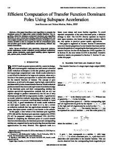
Fig. 1. Applying de Casteljau’s algorithm for bisecting a B´ezier curve of (3) degree 3. Note that p0 = B( 12 ), and the interior of the original curve B(t) for (0) (3) 0 < t < 12 is contained in the convex hull of p0 , . . . , p0 , while the interior (3) (0) 1 of B(t) for 2 < t < 1 is contained in the convex hull of p0 , . . . , p3 .

one over the domain 0 ≤ t ≤ τ , and the other over the domain (0) τ ≤ t ≤ 1. Let pk = pk for 0 ≤ k ≤ n, and recursively compute, for i = 1, 2, . . . , n and k = 0, 1, . . . , n − i: (i)

(i−1)

pk = (1 − τ )pk

(i−1)

+ τ pk+1 .

(2)

(n)

The point p0 obtained in the final stage equals B(τ ). Moreover, the subcurve of B over the domain 0 ≤ t ≤ τ is a B´ezier curve defined using the control points (0) (1) (2) (n) p0 , p0 , p0 , . . . , p0 , and the subcurve over τ ≤ t ≤ 1 is (n) (n−1) (n−2) (0) defined by p0 , p1 , p2 , . . . , pn . The de Casteljau algorithm provides a way to evaluate a point B(τ ) and its derivative along the curve, using basic arithmetic operations only. Especially note that if τ is rational then B(τ ) is a point with rational coordinates. Furthermore, it can be shown that if the curve is repeatedly subdivided, the resulting control polygons converge to the curve; see Figure 1 for an illustration. For a more thorough introduction to B´ezier curves and their properties see, e.g., [10]. In the rest of the paper, subdivisions are performed at τ = 12 , unless stated otherwise. C. Algebraic Number Types As we mentioned in the introduction, in order to handle non-linear curves in an exact manner, one needs to employ certified computation with algebraic numbers. A real number α is called algebraic if there exists a polynomial P(x) with integer (or, equivalently, rational) coefficients such that P(α ) = 0. We say that α is an algebraic number of degree d if d = deg(P), and α is not a root of any other integer polynomial with a smaller degree. The C ORE library9 [20] and the numerical facilities of L EDA10 [21, Chapter 4] provide number-types for operating on algebraic numbers. Namely, it is possible to compute the kth largest root of a polynomial with integer coefficients and to apply basic arithmetic operations (namely, +, −, × and ÷) on such roots. The computations are done in a certified manner, namely when we compare two algebraic numbers the result is guaranteed to be correct. Certified computation with algebraic numbers relies on the theory of separation bounds [22]. A major endeavor is to use as tight a separation bound as possible in order to expedite the computation; see, e.g., [23], [24]. Still, in many cases the estimated separation bounds are too small, incurring prohibitive running times. Thus, cascaded 9 http://www.cs.nyu.edu/exact/core/ . 10 http://www.algorithmic-solutions.com/enleda.htm .

4

SUBMITTED TO IEEE TRANSACTIONS ON AUTOMATION SCIENCE AND ENGINEERING

computations with the root operation — i.e., computing the root of a polynomial with algebraic coefficients — is either not supported (in C ORE), or is currently too slow for most practical purposes (in L EDA). The conic-traits class included in the arrangement package relies on C ORE to handle arcs of rational conic curves, namely algebraic curves of degree up to 2 with rational coefficients. As the intersection-point coordinates are in this case algebraic numbers of degree 4 at most, computations in this traits class are performed rather efficiently. Let us consider the case of B´ezier curves. As mentioned earlier, we assume that all control points have rational coordinates, so the endpoints of the input curves are rational points. However, these curves should be subdivided into x-monotone subcurves. Given a curve B(t) = (X(t),Y (t)), we compute the roots t1 < t2 < . . . < tk of X 0 (t) that lie in [0, 1], such that the x-monotone subcurves are defined over the parameter intervals [0,t1 ], [t1 ,t2 ], . . . , [tk , 1]. The endpoints of these intervals are given by B(ti ), where ti (1 ≤ i ≤ k) is an algebraic number of degree deg(B) − 1. Obtaining the intersection points between two B´ezier curves B1 (s) = (X1 (s),Y1 (s)) and B2 (t) = (X2 (t),Y2 (t)) is more involved. In this case we have to compute the roots of the following polynomial system: ½ X1 (s) = X2 (t) . (3) Y1 (s) = Y2 (t) This system of equations can be solved in the parameter space by calculating the roots of the resultant11 polynomials rest (X1 (t) − X2 (s),Y1 (t) −Y2 (s)), yielding the s-values, and ress (X1 (t) − X2 (s),Y1 (t) −Y2 (s)), which gives us the t-values. Only solution pairs of the form hs0 ,t0 i (i.e., B1 (s0 ) = B2 (t0 )), such that s0 ∈ [0, 1] and t0 ∈ [0, 1], are considered to be valid. Note that a B´ezier curve may also be self-intersecting. A self-intersection point occurs if there exists s0 ,t0 ∈ [0, 1] such that (X(s0 ),Y (s0 )) = (X(t0 ),Y (t0 )). If we denote X(t) = ∑nk=0 ξk t k and Y (t) = ∑nk=0 ηk t k , we have to solve the following system of polynomial equations: ½ n ∑k=1 ξk (t k − sk ) = 0 . ∑nk=1 ηk (t k − sk ) = 0 Note that all terms in the equation above are divisible by (t − s). Dividing by (t − s), we eliminate the trivial solution s = t and obtain the solutions for the following system: ¡ ¢ ½ n ∑k=1 ξk ¡∑ki=0 sit k−i ¢ = 0 . (4) ∑nk=1 ηk ∑ki=0 sit k−i = 0 The main problem is that the parameter-space solutions of Equation (3) are algebraic numbers of degree deg(B1 )·deg(B2 ) (and of degree (deg(B1 ) − 1)2 in case of a self-intersection). The complexity of the intersection-point coordinates, obtained by substituting these solutions into the curve equations, is even larger. As the efficiency of exact number-types quickly deteriorates as the degree of the number it handles increases, we try to avoid exact computations and only use them when absolutely necessary. 11 The resultant of two bivariate polynomials P (x, y) and P (x, y) with 1 2 respect to y, denoted resy (P1 , P2 ), is a univariate polynomial in x.

D. High-level Filtering Several arrangement traits-classes for algebraic curves have been developed as part of the E XACUS project [16], among them we mention a traits class for cubic curves [14], and another that handles special types of curves of degree four [15]. The traits classes consider only implicit algebraic curves, defined as the zero-set of some bivariate rational polynomial with bounded degree, namely curves given by the equation C(x, y) = 0, where C is a bivariate polynomial with rational coefficients. They apply algebraic filtering techniques to efficiently manipulate such curves. Instead of explicitly computing the intersection points, each point is isolated in some small bounding box with rational coordinates, where the boundaries of the box are computed by isolating the roots of a univariate rational polynomial whose roots are the xcoordinates of the intersection point (namely, the resultant polynomial resy (C1 ,C2 )). While algebraic filtering methods are very effective, they still make use of algebraic methods, such as resultant computation and univariate root-isolation involving polynomials with exact rational coefficients, which are applied to every pair of intersecting (or potentially intersecting) curves. In the case of the B´ezier traits class we use similar ideas, namely we isolate intersection points inside bounding boxes, but also take advantage of the geometric properties of B´ezier curves to construct these isolating boxes without applying any exact algebraic procedure whatsoever. III. T HE B E´ ZIER -T RAITS C LASS The implementation of our B´ezier-traits class consists of a layer that operates on bounding polygons, which serves as a filter for the exact algebraic layer. In this section we show how the representation of points and curves enables us to utilize the geometric properties of the B´ezier curves (e.g., the subdivision and convex-hull properties) such that the computationally demanding algebraic methods are mainly invoked for handling degenerate cases, where the geometric properties fail to give conclusive results. A. Representing Points and Curves In Section II-A we explained that any traits class must define the nested types Curve_2, X_monotone_curve_2 and Point_2. We next describe the structure of the nested types defined by our B´ezier-traits class. Curve_2: A B´ezier curve B is uniquely characterized by its control polygon. The curve class therefore stores the control points p0 , p1 , . . . , pn of B, that implicitly refer to the parameter domain t ∈ [0, 1]. The polynomials X(t) and Y (t) can be deduced from the control polygon at any time, according to Equation (1), and are therefore computed only when needed by applying “lazy evaluation”. Point_2: As explained in Section II-C, there are three types of points in our context: (i) input points with rational coordinates, (ii) split points of a curve into x-monotone subcurves, and (iii) intersection points. Points of the latter two types are characterized by some algebraic parameter value and their coordinates are algebraic numbers of a relatively high degree,

´ HANNIEL & WEIN: AN EXACT, COMPLETE AND EFFICIENT COMPUTATION OF ARRANGEMENTS OF BEZIER CURVES

thus computing them exactly is too costly for most practical applications. The point is therefore represented by a list of references to curves that are incident to it (the originating curves, or originators for short), coupled with the corresponding parameter value on each curve. The exact value of this parameter may not be known, as we explain next. Note that this representation can handle degenerate situations such as multiple curves intersecting at a point, or a coincidence of an endpoint and an intersection point. For every reference to an originating curve we also store a small control polygon, resulting from repeated subdivision of that curve around the point. The control polygon bounds the point on the curve in some parameter sub-domain [tlo ,thi ] (where thi − tlo = 2−m , m being the number of subdivisions performed on the original curve). Because of the convexhull property, the control polygon enables us to isolate the point by some small bounding box, namely the bounding box of its control points. The true coordinates of the point p are thus isolated in the intervals [xmin (p), xmax (p)] and [ymin (p), ymax (p)], respectively. The control polygon can be further refined upon request, yielding a tighter isolating box for the point. The exact algebraic coordinates of the point are evaluated only in a lazy manner to resolve ambiguities caused in degenerate or near-degenerate situations. X_monotone_curve_2: An x-monotone portion of a B´ezier curve is represented by references to its supporting curve (of type Curve_2) and to its endpoints. The usage of references makes it trivial, for example, to check whether two x-monotone subcurves originate from the same curve. B. Traits-Class Operations We next explain how the traits class implements the operations listed in Section II-A on objects of the types defined above. We begin by describing the construction operations, namely the subdivision of curves into x-monotone subcurves and the computation of intersection points, and then give details of the various predicates that involve the constructed objects, paying special attention to the fact that these objects are lazily evaluated. 1) Construction Operations: Make_x_monotone_2: Given a curve B(t) = (X(t),Y (t)) defined for t ∈ [0, 1], we can subdivide it into x-monotone subcurves by identifying all points B(t0 ) having a vertical tangent (namely X 0 (t0 ) = 0). As we wish to avoid the computation of the polynomial roots in a precise manner, we use the variation diminishing property of B´ezier curves, stating that an x-monotone control polygon guarantees that the curve is x-monotone. Thus, we recursively subdivide the curve B using de Casteljau’s algorithm, purging away subcurves with x-monotone control polygons. Furthermore, a convex y-monotone control polygon guarantees that there is a single vertical-tangency point on the curve, so we can terminate the subdivision when the subcurve has a y-monotone convex control polygon and isolate the vertical-tangency point within the bounding box of this polygon. In the remaining part of this section we consider only xmonotone B´ezier curves, characterized by a curve B(t) that is

5

defined on some continuous range of t-values. We denote such subcurves with the same notation used for their supporting curves. Intersect_2: To perform the parameter-space intersection of two curves B1 and B2 in a precise algebraic manner we have to compute the roots of the resultant polynomials res (X1 (s) − X2 (t),Y1 (s) −Y2 (t)), but this process is computationally expensive and we wish to avoid it whenever possible. We therefore use the subdivision and convex-hull properties of B´ezier curves to isolate intersection points. The idea is to isolate intersection points by recursively subdividing B1 and B2 , purging away subcurves that do not intersect by the convex-hull property. The subdivision termination criteria is based on the “bounding cones” of the curves [25]. Given a curve B(t) = (X(t),Y (t)), its bounding cone is the cone spanned by the angles of its derivatives B0 (t) = (X 0 (t),Y 0 (t)). The bounding cone is easy to compute for B´ezier and spline curves, since the tangent curve B0 (t) can be computed directly from the control polygon by taking the differences of the control polygon of B (p1 − p0 , p2 − p1 , . . . , pn − pn−1 ) as the control polygon of B0 (as we are only interested in the direction of the derivatives, we do not need to scale these differences by n, as explained in Section II-B). We can therefore easily compute the bounding cones of the two curves B1 and B2 and check whether they intersect only at the origin. If so, then the curves can intersect at most once (see [25] for the details). Otherwise, we have to bisect both curves using de Casteljau’s algorithm and continue recursively with the four pairs of subcurves we generate. In our implementation, we calculate the bounding cones of the relevant subcurves of B1 and B2 in each subdivision step. Once we obtain disjoint bounding cones we know that there can be at most one intersection point, and we just have to check whether such an intersection really exists. This is done by considering the skewed bounding boxes of the curves. A skewed bounding box of a curve is a bounding box oriented according to the line connecting the two curve endpoints. We say that a point is on the left (resp. right) of a skewed bounding box if it is to the left (resp. right) of both segments that are parallel to the line between the curve’s start and end points. See Figure 2(a) for an illustration. Proposition 1: Given two curves B1 and B2 and their skewed bounding boxes Σ1 and Σ2 , if the start and end points of B1 are on opposite sides of Σ2 (i.e., one is to the left and the other to the right of Σ2 ), and further, the start and end points of B2 are on opposite sides of Σ1 , then there must be at least one intersection of the curves within the area of intersection of the boxes. Figure 2(b) and (c) displays the idea of Proposition 1 on two B´ezier curves and their corresponding skewed bounding boxes. We check for the condition defined in Proposition 1 and if it is satisfied, we have isolated a single intersection point. Otherwise, we continue with the subdivision process. Given a skewed bounding box, checking whether the condition is satisfied can be done exactly using the orientation predicate. Computing the skewed bounding box of a subcurve is done by projecting its control points onto the line that connects the first point and the last point, then adding the largest projection

6

SUBMITTED TO IEEE TRANSACTIONS ON AUTOMATION SCIENCE AND ENGINEERING

B2 B1

b c

c(B2 )

p

p

c(B1 )

a d (a)

(b)

(c)

Fig. 2. (a) A B´ezier curve (solid line) given by three control points. The control polygon is drawn with a dashed line. The skewed bounding box of the curve is lightly shaded. Note that the point p is to the right of the box since it lies to the right of both lines supporting ab and dc. (b) Transversely intersecting B´ezier curves, shown with their control polygons and skewed bounding boxes. The axes-aligned isolating box of the intersection point p is drawn in a thin solid line. Note that the endpoints of B1 lie on opposite sides of the skewed bounding box of B2 and similarly the endpoints of B2 lie on opposite sides of the skewed bounding box of B1 (see Proposition 1). (c) The bounding cones of the curves.

vectors to the endpoints to get the corners of the skewed bounding box. The projection of a point on a line is a rational operation and can therefore be computed exactly using rational numbers. Having isolated an intersection point using two subcurves, we can construct a representation of the intersection point, bounding it in the skewed bounding box of the two intersecting subcurves, without the need to explicitly construct the resultant polynomials. While this geometric subdivision-based isolation procedure will terminate for transversal intersection, it will fail for degenerate tangential intersections. For these cases, the construction of the resultant and the computation of its roots is required. We therefore terminate the subdivision method and resort to the algebraic method when the subdivision passes some bound. The actual subdivision termination criteria depends on the implementation. For rational number types we terminate the subdivision at a user-defined bound. In the future, we plan to have an implementation of the traits class that uses interval arithmetic (see Section V). For such interval-arithmetic number types the criterion for subdivision termination will be when the bounding intervals do not enable a verified comparison. (Note that this means that the procedure of bounding the intersection points may also fail when there are two intersection points lying very close together.) 2) Traits-Class Predicates: As described in Section III-A, every point whose coordinates are not precisely known stores small control polygons, whose bounding box isolates the point coordinates. The Compare_x_2 predicate is therefore implemented as follows. Given two points p1 and p2 , check if xmax (p1 ) < xmin (p2 ) or whether xmin (p1 ) > xmax (p2 ), in which case we are done. Otherwise, we apply some refinement steps on the bounding boxes (see the previous subsection) until their x-ranges do not overlap any more. If we still fail, we either have a degeneracy, or a near-degeneracy that cannot be determined without using algebraic arithmetic. In this case we use the originators of each point to compute its exact representation, and perform an exact comparison to obtain a guaranteed result. Similar techniques also apply for the Compare_xy_2 predicate. The predicate Compare_y_at_x_2 is perhaps the most difficult to implement. Assume that we know that the point p is not on the x-monotone B´ezier curve B. We can then

subdivide the curve using de Casteljau’s algorithm until the bounding box of the control polygon (and hence the convex hull of the control polygon) is totally above or totally below the point p (or above/below the isolating box of this point). The convergence of the subdivision procedure guarantees that the procedure terminates. The difficulty lies in the fact that deciding whether a point p = (x0 , y0 ) is on a parametric B curve is not an easy task. For a rational point this amounts to extracting the root t0 of the polynomial X(t) − x0 = 0 that lies in the parameter range of B (recall that the curve is x-monotone, so there exists a unique solution with this property), and then checking whether Y (t0 ) = y0 . However, in case the point has algebraic coordinates, the free coefficient of X(t) − x0 = 0 is algebraic, and we cannot obtain an exact representation of the t-value (see the discussion in Section II-C). A possible solution is to implicitize the curve [17] and check whether the point (x0 , y0 ) satisfies the implicit representation. This process, however, requires to maintain the curve’s implicit representation after computing the resultant rest (X(t),Y (t)). This is a costly operation, as we usually try to avoid computing X(t) and Y (t) altogether. We therefore implemented a different approach, which checks for the intersection of the curve B with one of the originating curves of p. Let B p be the originating curve of p and s p be the parameter value such that p = B p (s p ) (recall that this information is stored with the point). If an intersection exists and one of the intersection parameters s of B p is identical to s p , then p is on B. To simplify the computation we choose B p as the minimal-degree originator of p. The drawback of this procedure is the need to intersect B and B p even if the construction of the arrangement does not require to intersect them (e.g., B and B p never become neighbors on the status line when applying the sweep-line algorithm). We therefore use the following strategy. First, we compare the bounding boxes of B and p and perform some refinement steps until we manage to separate their y-range, or until reaching our precision bound. If we manage to separate the bounding boxes, we can carry out the comparison quite cheaply. Otherwise we have to resort to exact methods and test whether p lies on B, as explained above. If it does, then we have a decisive result and we are done. Otherwise, we

´ HANNIEL & WEIN: AN EXACT, COMPLETE AND EFFICIENT COMPUTATION OF ARRANGEMENTS OF BEZIER CURVES

continue to refine the bounding boxes, this time using exact rational arithmetic with no precision bound. As p does not lie on B, this process will eventually yield the correct comparison result. The implementation of the Compare_y_at_x_right_2 predicate is also intricate when handling a degenerate case. We are given a point p, which is an intersection of B1 and B2 , such that B1 (s0 ) = B2 (t0 ). The parameter values s0 and t0 , or at least their approximate representation, are stored in p’s originator list. If p is a simple transversal intersection point of B1 and B2 , their order to the right of p can be easily determined by comparing the directions of the tangent vectors (X10 (s0 ),Y10 (s0 )) and (X20 (t0 ),Y20 (t0 )). The bounding-cones algorithm we use to isolate the intersection points also gives us a guarantee that these directions are well separated, even if s0 and t0 are only given as approximate intervals. In degenerate cases, we may have intersection points whose multiplicity is greater than 1. One can try comparing the curvatures of the curves, but this becomes cumbersome and for curves with the same curvature at p, a higher degree comparison is hard to formulate. We therefore use a different approach that makes use of the fact that sampling dense rational points on a parametric curve is relatively easy. We first check whether B1 and B2 intersect to the right of p or not. In the former case, we can compare the curves at a point between p and the nearest intersection point to the right of p. In the latter case, we can compare the curves at some point between p and the right endpoint that is closer to p. The comparison itself is done by choosing a rational point (x, ˆ y) ˆ on B1 and checking whether it is above or below B2 . This can be done by solving X2 (t) = xˆ and evaluating Y2 (tˆ) at the resulting parameter tˆ. IV. E XPERIMENTAL R ESULTS The running times reported in this section were obtained on a 3 GHz Pentium IV machine with 2 GB of R AM, running a Linux operating system. We have implemented two versions of a traits class that can handle B´ezier curves. The first employs the exact algebraic procedures described in Section II-C in all constructions and predicates, without using any geometric filtering. We refer to it as the “exact B´ezier-traits class”. The second class uses a filtering layer of bounding polygons to avoid exact algebraic computation, as described in Section III. In the filtering layer we employ exact rational computations, with a precision bound of 2−53 . We refer to this class as the “filtered B´ezier-traits class”. The first set of experiments we describe involves the construction of the arrangement of a set of B´ezier curves of degree 2, given by three control points. A degree 2 B´ezier curve is always a parabolic arc, and can thus be also represented by the traits class for conic arcs included in the arrangement package. Table I compares the construction times of arrangements of random parabolic arcs (the data sets contain 10, 20, 30 and 40 curves, respectively), each given by three control points within the unit square. The complexity of each arrangement (number of vertices, edges and faces) is also given in the table. Figure 3 shows two of the arrangements.

7

We compare the conic-traits class with the two versions of the B´ezier-traits class, the exact and the filtered one. The inferior performance of the conic-traits class is due to the fact that it has to compute the supporting parabola by considering five points on the curve, resulting in a rather complex representation. Also note that the gain achieved by filtering is not large in this case, as we only have to compute algebraic numbers of a relatively small degree. In order to compare our exact methods with traditional floating-point methods, we have also implemented a traits class that serves as a wrapper for the procedures that handle B´ezier curves in the I RIT modeling environment.12 I RIT performs all geometric operations using floating-point arithmetic, hence it is very fast compared to the exact methods we use. However, it may be instable in near-degenerate scenarios. For example, on the parabolas 40 random input (see Table I), the floating-point traits class produced incorrect results in some of the predicates, which caused the software to crash. Indeed, in this case we have a near-degenerate scenario, where our traits class needs to resort to exact computation for three different intersection points. The main feature of our scheme for handling B´ezier curves is that it produces topologically correct results in case of degeneracies. Consider for instance the example illustrated in Figure 5(a), where we have four curves (three parabolas and one line segment) all intersecting at a common point. Moreover, two of the parabolas are tangent to one another at this point. We are able to identify this degenerate situation and correctly construct the arrangement, which consists of 10 vertices, 12 edges and 4 faces in this case. The arrangement construction takes about 0.1 seconds. We can also successfully handle the degenerate scenario shown in Figure 5(b), where a B´ezier curve of degree 2 passes through the self-intersection point of a degree-3 curve. We are not aware of any other software that is capable of handling such degenerate configurations of B´ezier curves in a robust manner.

(a)

(b)

Fig. 5. (a) An arrangement induced by four B´ezier curves in degenerate position. (b) An arrangement containing a degenerate self-intersection point.

The effectiveness of filtering is emphasized when working with B´ezier curves of larger degrees. Table II shows the construction times of arrangements of B´ezier curves of degree 12 See, G. Elber, “The I RIT modeling environment”: http://www.cs.technion.ac.il/∼irit/ .

8

SUBMITTED TO IEEE TRANSACTIONS ON AUTOMATION SCIENCE AND ENGINEERING

(a)

(b)

Fig. 3. Arrangements induced by random parabolic arcs, given as B´ezier curves of degree 2: (a) the parabolas 20 data set, (b) the parabolas 40 data set. Points that are not computed in an exact manner and given by their bounding box are drawn as small circles. Other points (usually endpoints given as part of the input) are drawn as small discs. TABLE I C ONSTRUCTING THE ARRANGEMENTS OF RANDOM PARABOLAS USING DIFFERENT TRAITS CLASSES . T IMES ARE GIVEN IN SECONDS .

Input File parabolas parabolas parabolas parabolas

10 20 30 40

Arrangement |V | |E| 57 75 125 173 238 362 422 697

size |F| 20 51 127 277

I RIT floatingpoint traits 0.007 0.012 0.023 N/A

(a)

(b)

Conic-arc traits 20.149 57.407 126.024 232.315

Exact B´ezier traits 0.332 1.060 2.380 4.385

Filtered B´ezier traits 0.240 0.632 1.576 3.752

(c)

Fig. 4. Arrangements induced by sets of 10 B´ezier curves of different degrees: (a) degree 3, (b) degree 4 and (c) degree 5. Points that are not computed in an exact manner and given by their bounding box are drawn as small circles. Other points are drawn as small discs.

3 up to 5.13 In this case we used hand-drawn inputs, where the control points were all specified on the integer grid [0, 10000] × [0, 10000]. Each input file contains 10 B´ezier curves of the same degree. The induced arrangements are shown in Figure 4. Observe that the filtered B´ezier-traits class now runs 10–250 times faster than the exact B´ezier-traits class. Also note that the runtime overhead of using our filtered traits class, when compared to using the I RIT floating-point traits class, was reduced in Table II in comparison to Table I (10–25 times slower in Table II compared to 30–70 times 13 In the next set of experiments we also consider curves of degree 6. While the filtered B´ezier-traits class can efficiently handle curves of higher degrees, the running times for the exact traits class usually explode, so we do not bring experimental results with curves of higher degrees.

slower in Table I). The reason is that the input in Table I was given in floating-point numbers, which were converted to long rational numbers, whereas the input in Table II was given in integers. For the floating-point computations this did not make a difference, but for rational number types integer input is easier to handle. As we have already mentioned in the introduction, the arrangement package of C GAL serves as an infrastructure for several related packages, an important one being the Boolean set-operations package. That is, using our traits class we can compute regularized Boolean operations on general polygons whose boundaries are given as closed sequences of B´ezier curves. In our experiments we used characters taken from the Times

´ HANNIEL & WEIN: AN EXACT, COMPLETE AND EFFICIENT COMPUTATION OF ARRANGEMENTS OF BEZIER CURVES

(a)

(b)

9

(c)

Fig. 6. Computing the intersection of characters in the Times New Roman font: (a) A and V, (b) H and O, (c) m and g. The intersecting regions in each case are lightly shaded.

TABLE II C ONSTRUCTING THE ARRANGEMENTS OF B E´ ZIER CURVES OF HIGHER DEGREES . T IMES ARE GIVEN IN SECONDS .

Input File deg 3 deg 4 deg 5

Arrangement |V | |E| 40 47 52 64 50 59

size |F| 9 14 12

I RIT traits 0.004 0.016 0.020

Exact traits 1.220 7.916 51.079

Filtered traits 0.112 0.192 0.244

TABLE III C OMPUTING THE INTERSECTION OF T IMES N EW ROMAN CHARACTERS , ´ ZIER POLYGONS . T IMES ARE GIVEN IN SECONDS . GIVEN AS B E

χ1 (n1 ) A (23) H (48) S (35) m (52)

χ2 (n2 ) V (20) O (16) Z (15) g (43)

g (43)

s (29)

Result size {4, 4, 5} {21, 21} {6, 19, 24} {4, 11, 13, 6, 5, 9, 14, 5, 7} {31, 29}

Exact Tinit 0.105 0.195 0.382 0.402 0.360

traits Tcomp 17.4 174.9 367.7 543.6 737.8

Filtered Tinit 0.028 0.032 0.030 0.072

traits Tcomp 0.154 0.325 0.502 0.532

0.069

0.734

New Roman font. These characters are given as sequences of B´ezier curves of degrees 3 and 6 that specify the outer boundary of the characters and the boundary of the holes inside it (e.g., the character B has two holes, while V is simple and has no holes). In Table III we give the statistics of intersecting pairs of characters. For each pair χ1 , χ2 we give the number of curves that describe their boundaries (n1 and n2 , respectively), as well as the sizes of the general polygons that comprise the intersection χ1 ∩ χ2 . We use the exact B´ezier-traits class and the filtered traits class and compare the running times each class achieves. Figure 6 shows some of the character pairs we used in our experiments. Note that we separate between Tinit , the time needed to construct the two input polygons, and Tcomp , the time needed to compute the intersection by overlaying the two arrangements that correspond to χ1 and χ2 . While the filtered B´ezier-traits class performs the overlay 100–1000 times faster than the exact traits class, it also performs the initialization much faster. This is due to the fact that it does not construct the explicit polynomial representation of the B´ezier curve and just stores the sequence of control points per curve.

V. C ONCLUSIONS AND F UTURE W ORK We have presented a first implementation of a complete and robust arrangement of B´ezier curves of any degree. Our approach combines exact algebraic techniques with efficient methods based on the geometric properties of B´ezier curves. Thus, we manage to handle all degenerate and near-degenerate situations robustly, while maintaining a relatively low runtime overhead. We have shown the value and efficiency of our approach by comparing it to exact approaches and to traditional floating-point implementations. The usefulness of our work was demonstrated with a Boolean operation application on generalized polygons bounded by B´ezier curves. Our work is publicly available in the latest release of the C GAL library (Version 3.3.1). The work presented in this paper can be extended in several directions. The efficiency of the geometric filtering techniques can be improved by trying different representations of the curve’s control polygon. Currently we use the Cartesian kernel of C GAL with the G MP rational number-type for manipulating the control polygon. Implementing the geometric layer with different kernels that use filtering may speed up the computations in this layer. The geometric layer can also work with other number types. We plan to implement the geometric layer using interval arithmetic and extended floating point numbers, and we expect this to speed-up the application considerably, though there might be cases for which rational arithmetic will prove superior. The geometric algorithms used by the filtering layer may also be improved. Yap [26] has recently presented an adaptive subdivision algorithm for complete B´ezier curve intersection, which has similarities to the work described in this paper. The main difference is the use of of a geometric separation bound to terminate the subdivision without resorting to manipulation of algebraic numbers. We consider incorporating Yap’s algorithm in future implementations of the intersection function within our traits class. While a curve-intersection algorithm is a first step in constructing arrangements, other functions are also needed, as we have shown. Further research in the direction of geometric separation bounds may provide tools to reduce further the use of algebraic number-types in our application. Our implementation currently deals only with B´ezier curves. A natural extension of our application is the support of spline curves. Given a spline representation, we can construct an equivalent sequence of contiguous B´ezier curves (a B´ezier

10

SUBMITTED TO IEEE TRANSACTIONS ON AUTOMATION SCIENCE AND ENGINEERING

polycurve) through repeated knot insertion [10, Chapter 17]. Since knot insertion does not involve algebraic computations, this can be done in a straightforward manner. Thus, by preprocessing the input spline curves, our application can support arrangements of splines. Alternatively, since the spline representation has similar properties to B´ezier curves (e.g., the convex hull and the variation diminishing properties), we can implement the geometric filtering layer directly on the spline representation, and obtain the B´ezier polycurve representation only by lazy evaluation, when we have to resort to exact computation. Another extension is to implement arrangements of rational B´ezier curves. A rational B´ezier curve of degree n is defined by a sequence of n + 1 weighted control points, namely hp0 , w0 i, hp1 , w1 i, . . . , hpn , wn i as follows: B(t) = (X(t),Y (t)) =

n! · t k (1 − t)n−k ∑nk=0 wk pk · k!(n−k)! n! · t k (1 − t)n−k ∑nk=0 wk · k!(n−k)!

. (5)

Rational B´ezier curves are useful in many applications. In particular, they are used to represent conic sections. Since many of the geometric B´ezier properties that we use apply to rational B´ezier curves as well, the extension is natural. ACKNOWLEDGEMENTS The first author of this paper has been supported in part by the Israel Science Foundation (grant No. 857/04) and by European FP6 NoE grant 506766 (AIM@SHAPE). The second author has been supported in part by the IST Programme of the EU as Shared-cost RTD (FET Open) Project under Contract No IST-006413 (ACS - Algorithms for Complex Shapes), by the Israel Science Foundation (grant no. 236/06), and by the Hermann Minkowski–Minerva Center for Geometry at Tel Aviv University. The authors wish to thank Gershon Elber and Dan Halperin for their useful comments and encouragement. R EFERENCES [1] P. K. Agarwal and M. Sharir, “Arrangements and their applications,” in Handbook of Computational Geometry, J.-R. Sack and J. Urrutia, Eds. Elsevier Science Publishers B.V., 2000, pp. 49–119. [2] D. Halperin, “Arrangements,” in Handbook of Discrete and Computational Geometry, 2nd ed., J. E. Goodman and J. O’Rourke, Eds. Chapman & Hall/CRC, 2004, ch. 24, pp. 529–562. [3] C. M. Hoffmann, “Robustness in geometric computations.” J. Computing and Information Science in Engineering, vol. 1, no. 2, pp. 143–155, 2001. [4] C. K. Yap, “Robust geometric computation,” in Handbook of Discrete and Computational Geometry, 2nd ed., J. E. Goodman and J. O’Rourke, Eds. Chapman & Hall/CRC, 2004, ch. 41, pp. 927–952. [5] F. P. Preparata and M. I. Shamos, Computational Geometry: An Introduction. Springer, 1985. [6] S. Schirra, “Robustness and precision issues in geometric computation,” in Handbook of Computational Geometry, J.-R. Sack and J. Urrutia, Eds. Elsevier Science Publishers B.V., 2000, pp. 597–632. [7] R. Wein, E. Fogel, B. Zukerman, and D. Halperin, “Advanced programming techniques applied to CGAL’s arrangement package,” Computational Geometry: Theory and Applications, vol. 38, no. 1–2, pp. 37–63, 2007. [8] C. K. Yap and T. Dub´e, “The exact computation paradigm,” in Computing in Euclidean Geometry, 2nd ed., ser. Lecture Notes Series on Computing, D. Z. Du and F. K. Hwang, Eds. Singapore: World Scientific, 1995, vol. 1, pp. 452–492.

[9] E. Fogel, R. Wein, B. Zukerman, and D. Halperin, “2D regularized Boolean set-operations,” in C GAL-3.3 User and Reference Manual, C GAL Editorial Board, Ed., 2007, http://www.cgal.org/Manual/3.3/doc_html/cgal_manual/ Boolean_set_operations_2/Chapter_main.html. [10] E. Cohen, G. Elber, and R. F. Riesenfeld, Geometric Modeling with Splines: An Introduction. A. K. Peters, 2001. [11] M. Neagu and B. Lacolle, “Computing the combinatorial structure of arrangements of curves using polygonal approximations,” in Proc. 14th Europ. Workshop Comp. Geom. (EWCG), 1998. [12] I. Hanniel and D. Halperin, “Two-dimensional arrangements in CGAL and adaptive point location for parametric curves,” in Proc. 14th Workshop Alg. Eng. (WAE), 2000, pp. 171–182. [13] J. Keyser, T. Culver, D. Manocha, and S. Krishnan, “Efficient and exact manipulation of algebraic points and curves,” Computer-Aided Design, vol. 32, no. 11, pp. 649–662, 2000. [14] A. Eigenwillig, L. Kettner, E. Sch¨omer, and N. Wolpert, “Complete, exact and efficient computations with cubic curves,” in Proc. 20th Sympos. Comput. Geom. (SCG), 2004, pp. 409–418. [15] E. Berberich, M. Hemmer, L. Kettner, E. Sch¨omer, and N. Wolpert, “An exact, complete and efficient implementation for computing planar maps of quadric intersection curves,” in Proc. 21st Sympos. Comput. Geom. (SCG), 2005, pp. 99–106. [16] E. Berberich, A. Eigenwillig, M. Hemmer, S. Hert, L. Kettner, K. Mehlhorn, J. Reichel, S. Schmitt, E. Sch¨omer, and N. Wolpert, “EXACUS: Efficient and exact algorithms for curves and surfaces,” in Proc. 13th Europ. Sympos. Alg. (ESA), ser. LNCS, vol. 3669. Springer, 2005, pp. 155–166. [17] T. W. Sederberg and S. R. Parry, “Comparison of three curve intersection algorithms,” Computer Aided Design, vol. 18, no. 1, pp. 58–63, 1986. [18] M. H. Austern, Generic Programming and the STL: Using and Extending the C++ Standard Template Library. Addison-Wesley, 1998. [19] J. Snoeyink and J. Hershberger, “Sweeping arrangements of curves,” in Proc. 5th Sympos. Comput. Geom. (SCG), 1989, pp. 354–363. [20] V. Karamcheti, C. Li, I. Pechtchanski, and C. Yap, “A core library for robust numeric and geometric computation,” in Proc. 15th Sympos. Comput. Geom. (SCG), 1999, pp. 351–359. [21] K. Mehlhorn and S. N¨aher, L EDA: A Platform for Combinatorial and Geometric Computing. Cambridge University Press, 2000. [22] M. Mignotte, “Identification of algebraic numbers,” J. Algorithms, vol. 3, no. 3, pp. 197–204, 1982. [23] C. Burnikel, S. Funke, K. Mehlhorn, S. Schirra, and S. Schmitt, “A separation bound for real algebraic expressions,” in Proc. 9th Europ. Sympos. Alg. (ESA), 2001, pp. 254–265. [24] C. Li and C. Yap, “New constructive root bound for algebraic expressions,” in Proc. 12th Symp. Disc. Alg. (SODA), 2001, pp. 496–505. [25] T. W. Sederberg and R. J. Meyers, “Loop detection in surface patch intersections,” Computer Aided Geometric Design, vol. 5, no. 2, pp. 161–171, 1988. [26] C. K. Yap, “Complete subdivision algorithms I: Intersection of B´ezier curves,” in Proc. 22nd Sympos. Comput. Geom. (SCG), 2006, pp. 217– 226.

PLACE PHOTO HERE

Iddo Hanniel received his PhD. in computer science in 2008, from the Technion - Israel Institute of Technology. Prior to that he was a team leader and algorithm developer for five years at Proficiency Ltd. - an Israeli software company developing solutions for CAD interoperability. He received his MSc. in computer science from Tel-Aviv University in 2001. From 1997 to 2000 he was also the site technical coordinator of C GAL at Tel-Aviv University. His research interests include solid modeling, computational geometry and robust geometric computing.

PLACE PHOTO HERE

Ron Wein received his B.Sc. degree in mathematics and computer science from Tel-Aviv University in 1997, and his M.Sc. and Ph.D. degrees in computer science from the School of Computer Science, TelAviv University, Tel-Aviv, Israel, in 2002 and 2007, respectively. His research interests include robust geometric computation and its applications to fields like robotics and computer-aided design. Ron Wein is a member of the C GAL Editorial Board since 2005.