An Evolutionary Algorithm for Constrained Multiobjective Optimization Problems Ruhul Sarker , Hussein A. Abbass, and Samin Karim School of Computer Science, University of New South Wales, ADFA Campus, Northcott Drive, Canberra ACT, 2600, Australia, {r.sarker,h.abbass,s.karim}@adfa.edu.au

Presented at the 5th Australasia-Japan Joint Workshop University of Otago, Dunedin, New Zealand November 19 th -21st 2001 Abstract The use of evolutionary algorithms (EAs) to solve problems with multiple objectives (known as Multiobjective Optimization Problems (MOPs)) has attracted much attention recently. Population based approaches, such as EAs, offer a means to find a group of pareto-optimal solutions in a single run. However, most studies are undertaken on unconstrained MOPs. Recently, we developed the Pareto–frontier Differential Evolution (PDE) algorithm for unconstrained MOPs. The objective of this paper is to introduce a modification to PDE for handling constraints. The solutions, provided by the proposed algorithm for three test problems, are promising when compared with an existing well-known algorithm.

1 Introduction In Multi-objective optimization problems (MOPs), the aim is to simultaneously optimize a group of conflicting objectives. MOPs are a very important research topic, not only because of the multi-objective nature of most real-world decision problems, but also because there are still many open questions in this area. In fact, there is no universally accepted definition of optimum in MOPs as opposed to single-objective optimization problems, which makes it difficult to even compare results of one method to another. Normally, the decision about what the best answer is, corresponds to the so-called human decision maker (Coello 1999). Traditionally, there are several methods available in the Operational Research (OR) literature for solving MOPs as mathematical programming models, viz goal programming (Charnes and Cooper 1961), weighted sum method (Turban and Meredith 1994), goals as requirement (Coello 1999), and goal attainment (Wilson and Macleod 1993). Among these methods, goal programming is the most widely used in practice although it relies on domain knowledge to setup the goals’ aspiration levels. None of the previous methods treat all the objectives simultaneously which is a basic requirement in most MOPs. In MOPs, there is no single optimal solution, but rather a set of alternative solutions. These solutions are optimal in the wider sense that no other solutions in the search space are superior to (dominate) them when all objectives are simultaneously considered. They are known as pareto-optimal solutions. Pareto-optimality is expected to provide flexibility for the human decision maker. Recently, evolutionary algorithms (EAs) were found useful for solving MOPs (Zitzler and Thiele 1999). EAs have some advantages over traditional OR techniques. For example, considerations for convexity, concavity, and/or continuity of functions are not necessary in EAs, whereas, they form a real concern in traditional OR

techniques. MOPs are considered as difficult problems in the OR literature. The constrained MOPs are even more difficult. There exists many evolutionary computation based algorithms for solving unconstrained multiobjective (mainly with two objectives) optimization problems (Coello 1999). However, a few research have been carried out for constrained multiobjective optimization problems (CMOPs) with varying success (Binh and Korn 1997). In this paper, we extend our PDE algorithm for CMOPs. We compare its solutions for three benchmark problems with the algorithm of (Binh and Korn 1997), by using a statistical comparison technique recently proposed by Knowles and Corne (Knowles and Corne 1999; Knowles and Corne 2000). From the comparison, our algorithm performs better on these three test problems. The paper is organized as follows: background materials are scrutinized in Section 2 followed by the proposed algorithm in Section 3. Experiments are then presented in Section 4 and conclusions are drawn in Section 5.

2 2.1

Background Materials Multiobjective Optimization Problems Consider a MOP model as presented below:Optimize F (~x) subject to: Ω = {~x ∈ Rn |G(~x) ≤ 0 H(~x) = 0}

Where ~x is a vector of decision variables (x1 , . . . , xn ) and F (~x) is a vector of objective functions (f1 (~x), . . . , fK (~x)). Here f1 (~x), . . . , fK (~x), are functions on Rn and Ω is a nonempty set in Rn . The vectors G(~x) and H(~x) represent problem’s constraints. In MOPs, the aim is to find the optimal solution ~x∗ ∈ Ω which optimize F (~x). Each objective function, fi (~x), is either maximization or minimization. In this paper, we assume that all objectives are to be minimized for clarity purposes. We may note that any maximization objective can be transformed to a minimization one by multiplying it by -1. Unless the sub–objectives are highly positively correlated, a solution that is good for one is bad for another. Therefore, we need to define a partial order on the solutions, where a solution, ~x, is said to be a non–dominated solution, if there is no other solution, ~y , such that ~y is better than ~x on all objectives.

2.2

MOPs and EAs

EAs for MOPs (Coello 1999) can be categorized as plain aggregating, population-based non-Pareto and Pareto-based approaches. The plain aggregating approaches takes a linear combination of the objectives to form a single objective function (such as in the weighted sum method, goal programming, and goal attainment). This approach produces a single solution at a time that may not satisfy the decision maker, and it requires the quantification of the importance of each objective (eg. by setting numerical weights), which is very difficult for most practical situations. However optimizing all the objectives simultaneously and generating a set of alternative solutions, offer more flexibility to decision makers. The simultaneous optimization can fit nicely with population based approaches, such as EAs, because they generate multiple solutions in a single run.

The population-based approaches are more successful when solving MOPs, and are popular among researchers and practitioners. There are many algorithms for solving unconstrained two-objective optimization problems. These are Pareto Differential Evolution (PDE) algorithm (Abbass, Sarker, and Newton 2001), Multiobjective Evolutionary Algorithm (MEA) (Sarker, Liang, and Newton 2000), Strength Pareto Evolutionary Algorithm (SPEA) (Zitzler and Thiele 1999), Fonseca and Fleming’s genetic algorithm (FFGA) (Fonseca and Fleming 1993), Hajela’s and Lin’s genetic algorithm (HLGA)(Hajela and Lin 1992), Niched Pareto Genetic Algorithm (NPGA) (Horn, Nafpliotis, and Goldberg 1994), Non-dominated Sorting Genetic Algorithms (NSGA)(Srinivas and Dev 1994), Random Sampling Algorithm (RAND)(Zitzler and Thiele 1999), Single Objective Evolutionary Algorithm (SOEA) (Zitzler and Thiele 1999), Vector Evaluated Genetic Algorithm (VEGA) (Schaffer 1985) and Pareto Archived Evolution Strategy (PAES) (Knowles and Corne 1999; Knowles and Corne 2000). There are several versions of PAES like PAES, PAES20, PAES98 and PAES98mut3p. As mentioned earlier, there are a few evolutionary algorithms developed for constrained multiobjective optimization problems (Binh and Korn 1997; Binh 1999; Deb and Goel 2001). In constrained problems, the constraint handling is the additional task with the unconstrained problem. However, it is clear from the above discussions that unconstrained multiobjective algorithms are much more matured. The constraint handling in single objective is to some extent mature as will be discussed in a later sub-section. So, apparently, it seems that the proper marriage of constraint handling algorithms with unconstrained algorithms will provide a solution approach for constrained problems though it is not that simple. Binh and Korn (Binh and Korn 1997) proposed an algorithm for constrained multiobjective problems, which considers a degree of violation of constraints for infeasible solutions, in addition to the objective function vector, in selecting the potential parents. The infeasible individuals are ranked based on their degree of constraints violation. In (Deb and Goel 2001), a solution i is said to constrained-dominate a solution j, if any of the following conditions are true: 1. Solution i is feasible and j is not. 2. Both i and j are infeasible, but i has less constraint violation. 3. Both i and j are feasible and i dominates j. Here, feasible solutions constrained-dominate any infeasible solution and two infeasible solutions are compared based on their constraint violation only. However, when two feasible solutions are compared, they are checked based on their usual domination level. In this paper, we use a penalty approach, where a penalty value for constraint violation is added to each objective function.

2.3

Statistical Analysis

MOPs require multiple, but uniformly distributed, solutions to form a Pareto trade-off frontier. When comparing two algorithms, these two factors (the number of alternative solution points and their distributions) must be considered. There are a number of methods available in the literature to compare the performance of different algorithms. The error ratio and the generational distance are used as the performance measure indicators when the Pareto optimal solutions are known (Veldhuizen and Mamont 1999). The spread measuring technique expresses the distribution of individuals over the non-dominated region (Srinivas and Dev 1994). The method is based on a chi-square-like deviation distribution measure, and it requires several parameters to be estimated before calculating the spread indicator. The method of coverage metrics (Zitzler and Thiele 1999) compares the performances of different multiobjective evolutionary algorithms. It measures whether the outcomes of one algorithm dominate those of another without indicating how much better it is.

Most recently, Knowles and Corne (Knowles and Corne 2000) proposed a method to compare the performances of two or more algorithms by analyzing the distribution of an approximation to the Pareto–frontier. For two objective problems, the attainment surface is defined as the lines joining the points on the Pareto–frontier generated by an algorithm. Therefore, for two algorithms A and B, there are two attainment surfaces. A number of sampling lines can be drawn from the origin, which intersects with the attainment surfaces, across the full range of the Pareto–frontier. For a given sampling line, the intersection of an algorithm closer to the origin (for both minimization) is the winner. Given a collection of k attainment surfaces, some from algorithm A and some from algorithm B, a single sampling line yields k points of intersection, one for each surface. These intersections form a univariate distribution, and we can therefore perform a statistical test to determine whether or not the intersections for one of the algorithms occurs closer to the origin with some statistical significance. Such a test is performed for each of several lines covering the Pareto tradeoff area. Insofar as the lines provide a uniform sampling of the Pareto surface, the result of this analysis yields two numbers - a percentage of the surface in which algorithm A significantly outperforms algorithm B, and the percentage of the surface in which algorithm B significantly outperforms algorithm A.

2.4

Constraint Handling

Constrained optimization is a challenging research area in evolutionary computation (EC). Like conventional optimization techniques, the EC approaches have used penalty and barrier function concepts to handle constraints. Several penalty-function based genetic algorithms appear in the literature for single objective problems, namely static, dynamic, annealing, adaptive, death penalties and superiority of feasible points. The method of static penalties (Homaifar, Lai, and Qi 1994) uses a family of intervals for every constraint that determines the appropriate penalty coefficient. Joines and Houck (Joines and Houck 1994) propose dynamic penalties that vary with the generations. The method of annealing penalties, called GENOCOP II (for Genetic algorithms for Numerical Optimization of Constrained Problems), is also based on dynamic penalties and is described by Michalewicz and Attia (Michalewicz and Attia 1994) and (Michalewicz 1996). Adaptive transformation attempts to use the information from the search to adjust the control parameters. This is usually done by examining the fitness of feasible and infeasible members in the current population (Michalewicz and Schoenauer 1996). The death penalty method rejects infeasible individuals. The method of superiority of feasible points, developed by Powell and Skolnick (Powell and Skolnick 1993), is based on a classical penalty approach, with one notable exception. Each individual is evaluated by not only the objective and penalty function, but also by an additional iteration-dependent function that influences the evaluation of infeasible solutions. The point being that the method distinguishes between feasible and infeasible individuals by adopting an additional heuristic rule. In the penalty function method, infeasible solutions are penalized in each generation, and the overall penalty is added to the original objective function to form the fitness function for the evolutionary algorithms. The penalty is defined as follows:

φ(~x) =

m X

gj (~x)δj (~x)

(1)

j=1

where δj (~x) = 1, if gj (~x) > 0 and zero otherwise. Once φ(~x) = 0 for all parents in the population (ie. the entire population is feasible), the objective function fi (~x) is used alone during selection. The fitness function for objective fi corresponding to an individual ~x is ψ(~x) = fi (~x) + λφ(~x)

(2)

λ is a penalty parameter. For two objective problems with similar magnitude, there will be two fitness functions with the same penalty component λφ(~x).

2.5

Differential Evolution

Differential evolution (DE) is a branch of evolutionary algorithms developed by Rainer Storn and Kenneth Price (Storn and Price 1995) for optimization problems over continuous domains. In DE, each variable is represented in the chromosome by a real number. The approach works as follows:1. Create an initial population of potential solutions at random, where it is guaranteed, by some repair rules, that variables’ values are within their boundaries. 2. Until termination conditions are satisfied (a) Select at random a trial individual for replacement, an individual as the main parent, and two individuals as supporting parents. (b) With some probability, called the crossover probability, each variable in the main parent is perturbed by adding to it a ratio, F , of the difference between the two values of this variable in the other two supporting parents. At least one variable must be changed. This process represents the crossover operator in DE. (c) If the resultant vector is better than the trial solution, it replaces it; otherwise the trial solution is retained in the population. (d) go to 2 above. From the previous discussion, DE differs from genetic algorithms (GA) in a number of points: 1. DE uses real number representation while conventional GA uses binary, although GA sometimes uses integer or real number representation as well. 2. In GA, two parents are selected for crossover and the child is a recombination of the parents. In DE, three parents are selected for crossover and the child is a perturbation of one of them. 3. The new child in DE replaces a randomly selected vector from the population only if it is better than it. In simple GA, children replace the parents with some probability regardless of their fitness.

3

PDE: A Pareto–frontier Differential Evolution algorithm for MOPs

Abbass et al. (Abbass, Sarker, and Newton 2001) presented the Pareto-frontier Differential Evolution (PDE) algorithm for vector optimization problems. The algorithm is an adaptation of the DE algorithm described in the previous section with the following modifications:1. Assuming that all variables are bounded between (0,1), the initial population is initialized according to a Gaussian distribution N (0.5, 0.15). 2. The step-length parameter F is generated from a Gaussian distribution N (0, 1). 3. Reproduction is undertaken only among non-dominated solutions in each generation. 4. The boundary constraints are preserved either by reversing the sign if the variable is less than 0 or keeping subtracting 1 if it is greater than 1 until the variable is within its boundaries. 5. Offspring are placed into the population if they dominate the main parent.

The algorithm works as follows. Assuming that all variables are bounded between (0,1), an initial population is generated at random from a Gaussian distribution with mean 0.5 and standard deviation 0.15. All dominated solutions are removed from the population. The remaining non-dominated solutions are retained for reproduction. Three parents are selected at random (one as a main and also trial solution and the other two as supporting parents). A child is generated from the three parents and is placed into the population if it dominates the main parent; otherwise a new selection process takes place. This process continues until the population is completed. A maximum number of non-dominated solutions in each generation was set to 50. If this maximum is exceeded, the following nearest neighbor distance function is adopted: D(x) =

(min||x − xi || + min||x − xj ||) , 2

where x 6= xi 6= xj . That is, the nearest neighbor distance is the average Euclidean distance between the closest two points. The non-dominated solution with the smallest neighbor distance is removed from the population until the total number of non-dominated solutions is retained to 50.

4 4.1

Experiments Test Problems

The algorithm is tested on the following three benchmark problems. The first two problems and the third problem were collected from (Binh and Korn 1997) and (Binh 1999) respectively: Test Problem 1: f1 (x) = (x1 − 2)2 + (x2 − 11)2 + 2

(3)

f2 (x) = 9x1 − (x2 − 1)2

(4)

x21 + x22 − 255 ≤ 0

(5)

x1 − 3x2 + 10 ≤ 0

(6)

−20 ≤ xi ≤ 20, ∀i = 1, 2

(7)

Subject to

Test Problem 2: f1 (x) = 4x21 + 4x22 2

f2 (x) = (x1 − 5) + (x2 − 5)

(8) 2

(9)

Subject to (x1 − 5)2 + x22 − 25 ≤ 0

(10)

−(x1 − 8)2 − (x2 + 3)2 + 7.7 ≤ 0

(11)

−15 ≤ xi ≤ 30, ∀i = 1, 2

(12)

Test Problem 3: f1 (x) = −x21 + x2

(13)

f2 (x) = 0.5x1 + x2 + 1

(14)

Subject to x1 + x2 − 6.5 ≤ 0 6 0.5x1 + x2 − 7.5 ≤ 0

(15) (16)

5x1 + x2 − 30 ≤ 0

(17)

x1 , x2 ≥ 0

(18)

The computational results of these test problems are provided in the next section.

4.2

Experimental Setup

The initial population size is set to 100 and the maximum number of generations to 200. Eleven different crossover rates changing from 0 to 1.00 with an increment of 0.1 are tested without mutation. The initial population is initialized according to a Gaussian distribution N (0.5, 0.15). Therefore, with high probability, the Gaussian distribution will generate values between 0.5 ± 3 × 0.15 which fits with the variables’ boundaries. If a variable’s value is not within its range, a repair rule is used to repair the boundary constraints. The repair rule is simply to truncate the constant part of the value; therefore if, for example, the value is 3.3, the repaired value will be 0.3 assuming that the variable is between 0 and 1. The step-length parameter F is generated for each variable from a Gaussian distribution N (0, 1). The algorithm is written in standard C ++ and ran on a Sun Sparc 4.

4.3

Experimental Results and Discussions

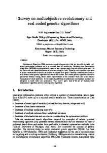
We obtained the solutions for all three test problems, produced by Binh and Korn’s algorithm, from Binh directly. To perform the statistical analysis using Knowles and Corne method (Knowles and Corne 2000), we used the solutions of the twenty runs for each crossover rate. The results of the comparison is presented in the form of a pair [a,b], where a gives the percentage of the space (i.e. the percentage of lines) on which algorithm A is found statistically superior to B, and b gives the similar percentage for algorithm B. For problem1, the best result [93.55,83.33] is achieved with crossover rate 0.70. This means, our algorithm outperforms Binh and Korn’s algorithm on about 93.55 percent of the Pareto surface whereas their algorithm is better than ours for 83.33 percent. For problem2, the best result [80.85,80.00] is obtained with crossover 0.90. The best result for problem3 is [100,0.0] at crossover rate 0.0. To show a sample analysis, the percentage outperformed by our algorithm and Binh and Korn’s algorithm are plotted against the crossover rate in Figure 1 for test problem 1. As we can see, our algorithm outperforms Binh and Korn’s algorithm for most crossover rates except 0.5 and 0.8. For illustration purposes, the followings are two points on the pareto frontier, Parameter x1 x2 f1 f2

Solution 1 2 11 2 -82

Solution 2 -4.816 15.225 66.312 -245.7

0.95 0.93

% Outperforms

0.91 0.89 PDE B&K

0.87 0.85 0.83 0.81 0.79 0

10

20

30

40

50

60

70

80

90

100

Crossover Rates

Figure 1: The performance of the PDE algorithm compared with Binh’s algorithm on the test problem 1. Crossover rates are in %.

5

Conclusions and Future Research

In this paper, a differential evolution based approach is presented for constrained optimization problems. The approach generates a step by crossover, where the step is randomly generated from a Gaussian distribution. We tested the approach on three benchmark problems and it was found that our approach is promising when compared to a standard approach from the literature. We also experimented with different crossover rates on these test problems to examine the performance. The crossover rates are found to be very sensitive to the solutions. For future work, we intend to test the algorithm on more problems. Also, the parameters chosen in this paper were generated experimentally. It would be interesting to see the effect of these parameters on the problem.

Acknowledgment We would like to thank T. Binh for providing us with the results of their algorithms.

References Abbass, H., R. Sarker, and C. Newton (2001). A pareto differential evolution approach to vector optimisation problems. Congress on Evolutionary Computation 2, 971–978. Binh, T. (1999). A multiobjective evolutionary algorithm: The study cases. In Technical report, Institute for Automation and Communication, Barleben, Germany. Binh, T. and U. Korn (1997). MOBES: A multiobjective evolution strategy for constrained optimization problems. In Proceedings of the third international Conference on Genetic Algorithms (Mendel97), Brno, Czech Republic, pp. 176–182.

Charnes, A. and W. Cooper (1961). Management models and industrial applications of linear programming, volume 1. John Wiley, New York. Coello, C. (1999). A comprehensive survey of evolutionary-based multiobjective optimization techniques. Knowledge and Information Systems 1(3), 269–308. Deb, K. and T. Goel (2001). Multi-objective evolutionary algorithms for engineering shape design. In R. Sarker, M. Mohammadian, and X. Yao (Eds.), Evolutionary Optimization. Kluwer Academic Publishers, USA. Fonseca, C. and P. Fleming (1993). Genetic algorithms for multiobjective optimization: Formulation, discussion and generalization. Proceedings of the Fifth International Conference on Genetic Algorithms, San Mateo, California, 416–423. Hajela, P. and C. Lin (1992). Genetic search strategies in multicriterion optimal design. Structural Optimization 4, 99–107. Homaifar, A., S.-Y. Lai, and X. Qi (1994). Constrained optimization via genetic algorithms. Simulation 62(4), 242–254. see also paper by Fogel the following year (same journal). Horn, J., N. Nafpliotis, and D. Goldberg (1994). A niched pareto genetic algorithm for multiobjective optimization. Proceedings of the First IEEE Conference on Evolutionary Computation 1, 82–87. Joines, J. and C. Houck (1994). On the use of non-stationary penalty functions to solve nonlinear constrained optimization problems with GAs. In Z. et al.. Michalewicz (Ed.), IEEE International Conference on Evolutionary Computation, pp. 579–584. IEEE Press. Knowles, J. and D. Corne (1999). The pareto archived evolution strategy: a new baseline algorithm for multiobjective optimization. In 1999 Congress on Evolutionary Computation, Washington D.C., IEEE Service Centre, 98–105. Knowles, J. and D. Corne (2000). Approximating the nondominated front using the pareto archived evolution strategy. Evolutionary Computation 8(2), 149–172. Michalewicz, Z. (1996). Genetic algorithms + data structures = evolution programs (3rd ed.). New York: Springer Verlag. Michalewicz, Z. and N. Attia (1994). Evolutionary optimization of constrained problems. In A. Sebald and L. Fogel (Eds.), Annual Conference on Evolutionary Programming, pp. 98–108. World Scientific Publishing. Michalewicz, Z. and M. Schoenauer (1996). Evolutionary algorithms for constrained parameter optimization problems. Evolutionary Computation 4(1), 1–32. Powell, D. and M. Skolnick (1993). Using genetic algorithms in engineering design optimization with nonlinear constraints. In S. Forrest (Ed.), Proc. of the 5th Int. Conf. on Genetic Algorithms, pp. 424–0430. San Mateo, CA: Morgan Kaufmann. Sarker, R., K. Liang, and C. Newton (2000). A multiobjective evolutionary algorithm. Proceedings of the Computational Intelligence (CI’2000), International ICSC Congress on Intelligent Systems & Applications 2, 125–131. Schaffer, J. (1985). Multiple objective optimization with vector evaluated genetic algorithms. Genetic Algorithms and their Applications: Proceedings of the First International Conference on Genetic Algorithms, 93–100. Srinivas, N. and K. Dev (1994). Multiobjective optimization using nondominated sorting in genetic algorithms. Evolutionary Computation 2(3), 221–248. Storn, R. and K. Price (1995). Differential evolution: a simple and efficient adaptive scheme for global optimization over continuous spaces. Technical Report TR-95-012, International Computer Science Institute, Berkeley. Turban, E. and J. Meredith (1994). Fundamentals of Management Science. McGraw-Hill, Boston, USA.

Veldhuizen, D. V. and G. Mamont (1999). Multiobjective evolutionary algorithm test suites. Procedings of the 1999 ACM Sysposium on Applied Computing, San Antonio, Texas, ACM, 351–357. Wilson, P. and M. Macleod (1993). Low implementation cost iir digital filter design using genetic algorithms. IEE/IEEE workshop on Natural Algorithms in Signal Processing, 1–8. Zitzler, E. and L. Thiele (1999). Multiobjective evolutionary algorithms: A comparative case study and the strength pareto approach. IEEE Transactions on Evolutionary Computation 3(4), 257–271.