AN EMPIRICAL STUDY OF LEARNING RATES IN DEEP NEURAL NETWORKS FOR SPEECH RECOGNITION Andrew Senior, Georg Heigold, Marc’Aurelio Ranzato, Ke Yang Google Inc., New York {andrewsenior,heigold,ranzato,yangke} @google.com ABSTRACT Recent deep neural network systems for large vocabulary speech recognition are trained with minibatch stochastic gradient descent but use a variety of learning rate scheduling schemes. We investigate several of these schemes, particularly AdaGrad. Based on our analysis of its limitations, we propose a new variant ‘AdaDec’ that decouples long-term learning-rate scheduling from per-parameter learning rate variation. AdaDec was found to result in higher frame accuracies than other methods. Overall, careful choice of learning rate schemes leads to faster convergence and lower word error rates. Index Terms— Deep neural networks, large vocabulary speech recognition, Voice Search, learning rate, AdaGrad, AdaDec. 1. INTRODUCTION The training of neural networks for speech recognition dates back to the 1980s but has recently enjoyed a resurgence as several groups [1, 2] have demonstrated striking performance improvements relative to previous state-of-the-art Gaussian mixture model (GMM) systems for large vocabulary speech recognition. Across these systems the fundamental architecture is the same — a network consisting of several hidden layers l of neurons i whose activations hi (l) are a nonlinear function of a linear combination of the activations, hj (l  − P 1), of the previous layer, l − 1: hi (l) = σ w h (l − 1) , ij j j where σ is a sigmoid function and the final layer uses a softmax [3] to estimate the posterior probability of each speech state. These probabilities are used in a Hidden Markov Model (HMM) speech recognizer to find a text transcription of speech. In the next section we outline stochastic gradient descent and describe the methods used to determine the learning rate, including the new “AdaDec” variant. In the following section we describe our speech recognition task and experimental set-up. In the subsequent sections we present our experiments into learning rate scheduling and finish with conclusions. 2. STOCHASTIC GRADIENT DESCENT Gradient descent learning algorithms attempt to minimize the loss L of some function approximator by adapting the parameters {wij } with small increments proportional to an estimate of the gradient ∂L . The constant of proportionality is termed the learning gij = ∂w ij rate, η. Algorithms may estimate the gradient on a large dataset (batch), or on a single example (Stochastic Gradient Descent: SGD). While the gradients from SGD are by their nature noisy, SGD has been shown to be effective for a variety of problems. In this paper we focus on minibatch SGD where an average gradient is estimated on a

small sample of τ examples called a minibatch. So, after presenting t frames of data: wij (t) = wij (t − τ ) − ηˆ gij (t) (1) gˆij (t)

=

τ −1 1 X gij (t − t0 ). τ 0

(2)

t =0

τ = 200 for all the experiments described in this paper. There is much current research into second order optimization methods [4, 5, 6] for neural networks, but the majority of work still uses the fast, simple stochastic gradient descent algorithm, and we focus on this algorithm here. Momentum can improve convergence, particularly later in training. Here momentum was set to 0.9 throughout all the experiments. 2.1. Learning rate scheduling It is well known that reducing the step size is essential for proving convergence of SGD [12] and helps in practical implementations of SGD. A good schedule that changes the learning rate over time can result in significantly faster convergence and convergence to a better minimum than can be achieved without. Initial large steps enable a rapid increase in the objective function but later on smaller steps are needed to descend into finer features of the loss landscape. While several groups [2, 7, 8, 9, 10] have adopted a similar approach to training speech models, we find that each has taken a different approach to learning rate scheduling. There have also been attempts to automate the setting of learning rates [11]. In our work we explored the following different methods of learning rate scheduling: • Predetermined piecewise constant learning rate. This method has been used in the successful training of deep networks for speech [13, 10] but clearly has limitations in that it is difficult to know when to change the learning rate and to what value. • Exponential Scheduling: We have also explored exponential scheduling where the learning rate decays as: η(t)

=

η(0) × 10−t/r

(3)

• Power Scheduling: Bottou [14] follows Xu [15] in using a decaying learning rate of the form: η(t) = η(0)(1 + t/r)−c (4) Where c is a “problem independent constant” (Bottou uses 1 for SGD and 0.75 for Averaged SGD). • Performance Scheduling: A further option that has long been used in the neural network community [16, 7] is to base parameter schedules on some objective measure of performance, e.g. reducing the learning rate when smoothed frame accuracy or cross-entropy does not improve.

• AdaGrad [17] is an alternative algorithm for managing the learning rate on a per-parameter basis, thus determining a long-term decay and a per-parameter variation akin to that of second-order-methods. In this case the learning rate ηij (t) for each parameter, wij is decayed according to the sum of the squares of the gradients: ηij (t)

=

η(0) p P K + t gˆij (t)2

(5)

Following [8] we add an initialization constant K to ensure that the learning rate is bounded and in practice choose K = 1 to ensure that AdaGrad decreases the learning rate. In that work, AdaGrad of this form has been found to improve convergence and stability in distributed SGD. • AdaDec: We propose a variant of AdaGrad with a limited memory wherein we decay the sum of the squares of the gradients over time to make the learning rate dependent only on the recent history. Naturally this decaying sum will not continue to increase in the same way as the AdaGrad denominator will, so we also multiply by a global learning rate from one of the schedules above, which allows us to control the long-term decay of the learning rate while still making the learning rate of each parameter depend on the recent history of the gradient for that parameter. η(t) K + Gij (t)

ηij (t)

=

p

Gij (t)

=

γGij (t − τ ) +

(6) τ −1 1 X gˆij (t − t0 )2 τ 0

(7)

t =0

with η(t) given by the power scheduling equation 4. γ = 0.999 was used here. • In RProp [18] and the extended family of algorithms including iRProp+/- [19] each element of the gradient has a separate learning rate which is adjusted according to the sign of the gradients. If the sign is consistent between updates then the step size is increased, but if the sign changes, the step size is decreased. RProp is sensitive to changes in the gradient between batches, so is unsuited to minibatch SGD, though it has been shown to work well for batches 1000 times larger than those used for SGD [20]. We tried without success to adapt it to work with smaller sample sizes so present no results for RProp or its variants. 3. VOICE SEARCH TASK Google Search by Voice is a service available on several mobile phone platforms which allows the user to conduct a Google search by speaking a query. Google Voice Input Method Editor (IME) allows the user to enter text on an Android phone by speaking. Both systems are implemented “in the cloud”, falling-back to an on-device recognizer for IME when there is no network connection. 3.1. Data For our experiments we trained speech recognition systems on 3 million anonymized and manually transcribed utterances taken from a mix of live VoiceSearch / Voice IME traffic and test on a similar set of 27,000 utterances. The speech data is represented as 25ms frames of 40 dimensional log filterbank energies calculated every 10ms. The entire training set is 2750 hours or 1 billion frames from which we

hold out a 200,000 frame development set for frame accuracy evaluation. A window of consecutive frames is provided to the network as input. Deep networks are able to exploit higher dimensionality data and thus longer windows than GMMs. We limit the number of future frames to 5 since increasing the number of future frames increases the latency, which is of critical concern for our real-time application. We take 10 frames of past acoustic context to keep the total number of parameters low, so the network receives features from 16 consecutive frames, i.e. 175ms of waveform, at each frame. 3.2. Evaluation The word error rate (WER) is a good measure of the performance of a dictation system, and a reasonable approximation of the success of a voice search system (which may return useful results despite transcription errors). We evaluate WERs in this paper and our goal is to achieve the lowest WER for our task. However, the networks trained here optimize a frame-level cross entropy error measure which is not directly correlated with WER. For simplicity of comparison of networks during training we present the Frame Accuracy which is the proportion of the development set frames which are correctly classified by the network. This is found to behave similarly to the cross entropy. The frame classifcation involves no sequence level information. It is difficult to compare across systems with different numbers of outputs or indeed across different datasets, since the results here are dominated by the three silence states which contribute 30% of the frames in the development set. Unfortunately the initial convergence rate for a given scheme or experiment does not necessarily indicate the final converged frame accuracy, the time taken to reach convergence, nor the final WER. Where possible we have allowed networks to continue training until frame accuracies have levelled off, or where frame accuracy is clearly not going to exceed that of another method within a reasonable time We show experiments on networks trained for up to 20 epochs. 3.3. GPU Trainer The networks in this paper are trained using a Graphics Processing Unit (GPU)-based training system [10] using CUBLAS through the CUDAMat library [21], extended with many custom kernels. Each network is trained on a single GPU (mostly NVIDIA GeForce GTX580) and we rely on the GPU’s fast parallel floating point operations, particularly matrix multiplication, for fast training, with no CPU-GPU transfers except to load training data and save final trained network parameters. The system can train the networks described here at about 35,000 frames per second, or three epochs/day. 3.4. Deep neural network system The networks used for these experiments all have 1.6 million parameters: an input window of 10 past + 1 current + 5 future 40dimensional frames, four hidden layers of 480 sigmoid units and 1000 softmax outputs. This configuration is chosen to be sufficiently small for inference and large vocabulary speech decoding to run faster than real time on a modern smartphone, based on extensive previous work to optimize evaluation speed for both server and embedded implementations, by exploiting 8-bit quantization, SIMD instructions, batching and lazy evaluation [22]. The neural networks are randomly initialized and trained by minibatch stochastic gradient descent to discriminate between the state labels, minimizing a cross-entropy criterion. Initial forced alignments of the data came from a 14247 state Gaussian Mixture model with 616,335 Gaussians trained from scratch on the data. This baseline model achieved 15.0% WER

1e-01 Learning rate

Performance Power Exponential

1e-02

55 54.5

1e-04 0

5

10

15

20

Frame Accuracy

56 55 54 53

Performance Power Exponential Constant

52 51 0

5

10 Training frames x 1e9

15

Frame Accuracy

1e-03 54 53.5 Power schedule AdaGrad 0B AdaGrad 1B Adagrad 2B AdaGrad 3B AdaGrad 3B 3x AdaGrad 4B Step change 0.25x 3B

53 52.5

20

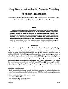
Fig. 1: Frame accuracy and learning rate against number of training frames for a constant learning rate and Performance, Power and Exponential scheduling. on the test set. A large (68M parameter) deep network model was trained on this data, and achieved 10.7% WER. This was then used to create a new alignment. The context dependency trees (rooted in 126 context independent states) were pruned back according to a maximum likelihood criterion, until there were 1000 CD states. The large network’s alignment was then relabelled to the smaller state inventory and used to train the small networks shown in this work, resulting in more accurate alignments than starting from a system with only 1000 states. Realigning gave faster convergence in terms of both frame accuracy and WER. 4. EXPERIMENTS Figure 1 shows a comparison between the basic global learning rate scheduling schemes, comparing a constant learning rate (η = 0.04) with power scheduling (η(0) = 0.08, r = 250, 000, 000) and performance scheduling, using the optimal parameters found for each scheme in other experiments. In Performance Scheduling we multiplied the learning rate by a decay rate (0.95) if the frame accuracy did not increase within a window of E evaluations (E = 50 with evaluations every 1,000,000 frames) and found that despite initial slow convergence this eventually resulted in high frame accuracies. The curve tends to flattens out completely as learning rates become so small that performance does not change — gains in accuracy become rarer as the curve flattens out, triggering more learning rate reductions. Initially the learning rate does not change since the accuracy is increasing steeply. Unfortunately Performance Scheduling has several hyper-parameters (the decay rate and the window size, as well as the frequency of the evaluations) as well as the tendency to decay the learning rate too much at the end, and to not change it at all at the beginning. Based on the behaviour of Power and Performance scheduling, and observing the opposite curvatures of the learning rate curves for the two schemes, shown in Figure 1, we tried Exponential scheduling — a straight line in the figure, characterized by a single hyperparameter. Here r = 6.6 × 109 . Ultimately a higher frame accuracy was achieved than with any of the other schemes, though convergence took significantly longer. 4.1. AdaGrad In our experiments, shown in Figure 2, we found that beginning training with AdaGrad (“AdaGrad 0B”) led to poor convergence. Increasing the learning rate a factor of 3–5 improved things, but not close to the performance of Power Scheduling. Starting AdaGrad from a partially-trained model produced a large initial increase in

52 0

2

4

6 8 10 Training frames x 1e9

12

14

Fig. 2: Frame accuracy for AdaGrad, from random initialization (0B) or initializing from the power scheduling model after 1, 2, 3, and 4 billion frames. After an initial step, performance flattens off and is soon surpassed by Power Scheduling. Similar behaviour is seen without AdaGrad if the learning rate is divided by four. At a given number of frames, the most recent warm start performs best. Increasing the learning rate helps with random initialization, but hurts (“AdaGrad 3B 3x” curve) when warm-starting. frame accuracy. However the frame accuracy of PowerScheduling increases at a faster rate, and as shown in Figure 2, in all circumstances it soon surpasses the AdaGrad training. Increasing the learning rate reduced the initial performance step, and did not change the slope of the curve. The sharp increase in frame accuracy is partly attributable to the parameter-specific learning rates, but we suggest that it is principally due to a rapid decrease in the learning rate for all the parameters. As shown in the figure, a step change in the global learning rate produces a similar step change and reduced slope for the frame accuracy curve. Figure 3a shows the percentiles of the learning rate for one layer of the network compared to the power scheduling. The median learning rate from AdaGrad starts out 10× lower than the global η but soon falls to 30× lower. Increasing the learning rate to compensate merely reduced the initial gain from AdaGrad. We note that there is a wide separation (265×) between the maximum and minimum learning rate, but only a small separation (around 2.7×) between the 10th and 90th percentiles. Increasing the learning rate to compensate when warm-starting AdaGrad reduced the step change but did not improve the slope of the curve (Figure 2). Another reason that we can propose for AdaGrad’s poor performance, particularly when used at the start of training, is that it has an unlimited memory. The early history of a gradient sequence impacts the learning rate long after, when the gradient behaviour may be very different. A further drawback of AdaGrad is the extra computation: AdaGrad reduces the frame throughput by about 13 . 4.2. AdaDec To address these problems we propose a variant — AdaDec, described in Equations 6 and 7 in which we decouple the per-parameter learning rate estimation from the time-dependent learning rate decay. Figure 3b shows the change in the learning rate multiplier from AdaDec over time, with a smaller range (50×) from maximum to minimum, but a similar range for the middle 80% of learning rates, and a relatively stable median. We can apply AdaDec with the global learning rate schedule of our choice. As with AdaGrad, we initially compared to Power Scheduling, with frame accuracies shown in Fig-

55.7 1

0.001

0.0001

1e-05

Frame Accuracy

0.01

Max 90% Median 10% Min

0.1

2

3

4

5

6

55.5

Power Performance Exponential Exp + AdaDec 13B x6 Exp + AdaDec 14B x6 + Av_av

55.4 55.3 55.2 55.1 6

0.01 1

55.6

55

1

2

Training Frames x1e9

3

4

5

6

Training Frames x1e9

(a)

(b)

Fig. 3: Percentiles of the learning rates for the penultimate layer against number of training frames, initializing at 1 billion frames. (a) AdaGrad compared to Power Scheduling. The maximum learning rate decreases rapidly then roughly parallels the Power Scheduling curve a factor of 4.4 lower. The dynamic range is about 265, (2.7 for the middle 80%). (b) AdaDec, excluding the global scaling factor. (Max≈ 1). The median falls from 0.31 to 0.25. The dynamic range of the learning rates is around 50, with a similar spread to AdaGrad (2.6) for the middle 80%. ure 4. There is the same immediate step change in the frame accuracy as seen with AdaGrad, but the frame accuracy increases more rapidly, albeit still being caught by the Power Scheduling frame accuracy. Again it seems better to warm-start later rather than sooner. When the learning rate is increased, the step change is smaller but AdaDec frame accuracies rise and exceed the Power Scheduling for the scope of the experiment. 55.2

WER

Power scheduling Max 90% Median 10% Min

Learning rate (log scale)

Learning rate (log scale)

0.1

8

10

12

14

15.1 15 14.9 14.8 14.7 14.6 14.5 14.4 14.3 14.2

16

18

20

18

20

Power Performance Exponential

6

8

10 12 14 Training frames x 1e9

16

Fig. 5: Comparison of frame accuracies against training frames for Power Scheduling, Performance scheduling, Exponential scheduling and Exponential scheduling with a late AdaDec warm start, with and without model averaging. The WERs for each of the global schemes are shown. AdaDec achieves the same 14.3% WER, slightly later than the simple Exponential model. ing rates every M batches. With N = 3, M = 9 the frame rate drop from applying AdaGrad is only 13%. As with AdaGrad, we find that at any given training frame, the most recently started AdaDec model achieves the highest frame accuracy, so Figure 5 also shows the result of starting AdaDec at 13& 14 billion frames. Finally we apply a model averaging [23] with a running average [15] which increases the frame accuracy slightly but has had no measurable effect on the final WER. 5. CONCLUSIONS

Frame Accuracy

55

54.8

54.6

AdaDec 4B AdaDec 3B x3 AdaDec 3B AdaDec 2B AdaDec 1B AdaGrad 4B AdaGrad 3B Adagrad 2B AdaGrad 1B Power schedule

54.4

54.2

54 0

5

10 Training frames x 1e9

15

20

Fig. 4: Frame accuracies comparing AdaGrad with AdaDec with the same initial global learning rate, starting at each of 1, 2, 3, 4 billion frames. Power Scheduling is shown for comparison. Increasing the learning rate by a factor of 3 when starting AdaDec (black dots) results in sustained outperformance of PowerScheduling. When we apply AdaDec to an exponential schedule, we find the same step improvement and, when the learning rate is increased, a sustained improvement relative to the exponential schedule. Earlier in training, where the gap in frame accuracies is large, AdaDec results in improved WER, however, where the gap is small we did not measure any improvement, and in fact measured by time, rather than number of frames processed, AdaDec reached the optimum WER later than exponential scheduling. To this end we propose a further improvement to AdaDec, which is to only accumulate the sum of squared gradients every N batches and to only recompute the learn-

Learning rate scheduling is essential to achieving optimal WER from deep neural networks. Careful choice of the learning rate scheduling algorithm and the hyperparameters can result in dramatically different training times for current network trainers using minibatch stochastic gradient descent, and different WER, particularly when training with a limited computation budget. The space of parameter schedules is infinite, and many previous studies have explored parameter scheduling for other problems (SGD, ASGD, convex problems etc.) For our task, we find the self-regulating performance scheduling to be effective, but more complex and with more hyperparameters than the exponential scheduling that ultimately achieves the best performance. In particular we have studied AdaGrad and found no practical improvement. Based on our findings we have designed AdaDec, an alternative which is shown to produce faster convergence to higher frame accuracies for our task. Ultimately our study has led to a 0.2% reduction in the WER for the system investigated below the previous best. 6. ACKNOWLEDGEMENTS We would like to thank Geoff Hinton and Matt Zeiler for productive discussions about AdaGrad variants. 7. REFERENCES [1] G.E. Dahl, D. Yu, L. Deng, and A. Acero, “Large vocabulary continuous speech recognition with context-dependent DBNHMMs,” in ICASSP, 2011. [2] G. Hinton, L. Deng, D. Yu, G. Dahl, A. Mohamed, N. Jaitly, A. Senior, V. Vanhoucke, P. Nguyen, T. Sainath, , and B. Kings-

bury, “Deep neural networks for acoustic modeling in speech recognition,” IEEE Signal Processing Magazine, vol. 29, no. 6, November 2012.

[20] M. Mahajan, A. Gunawardana, and A. Acero, “Training algorithms for hidden conditional random fields,” in ICASSP, 2006, pp. 273–276.

[3] J.S. Bridle, “Training stochastic model recognition algorithms as networks can lead to maximum mutual information estimation of parameters,” in NIPS, 1990, vol. 2, pp. 211–217.

[21] V. Mnih, “CUDAMat: A CUDA-based matrix class for Python,” Tech. Rep. 2009-004, University of Toronto, Nov. 2009.

[4] T. LeCun, L. Bottou, G. Orr, and K. Muller, “Efficient backprop,” in Neural Networks: Tricks of the trade, G. Orr and Muller K., Eds. Springer, 1998.

[22] V. Vanhoucke, A. Senior, and Mao M., “Improving the speed of neural networks on CPUs,” in NIPS Workshop on deep learning, 2011.

[5] B. Kingsbury, T.N. Sainath, and H. Soltau, “Scalable minimum bayes risk training of deep neural network acoustic models using distributed hessian-free optimization,” in Interspeech, 2012.

[23] B.T. Polyak and A.B. Juditsky, “Acceleration of stochastic approximation by averaging,” Automation and Remote Control, vol. 30, no. 4, pp. 838–855, 1992.

[6] O. Vinyals and D. Povey, “Krylov subspace descent for deep learning,” in NIPS Deep learning workshop, 2011. [7] T. N. Sainath, B. Kingsbury, B. Ramabhadran, P. Fousek, P. Novak, and A. Mohamed, “Making deep belief networks effective for large vocabulary continuous speech recognition,” in ASRU, December 2011. [8] J. Dean, G. S. Corrado, R. Monga, K. Chen, M. Devin, Q. V. Le, M. Z. Mao, M.’A. Ranzato, A. Senior, P. Tucker, K. Yang, and A.Y. Ng, “Large scale distributed deep networks,” in NIPS, 2012. [9] F. Seide, G. Li, and D. Yu, “Conversational speech transcription using context-dependent deep neural networks,” in Interspeech, 2011. [10] N. Jaitly, P. Nguyen, A. W. Senior, and V. Vanhoucke, “Application of pretrained deep neural networks to large vocabulary speech recognition,” in Interspeech, 2012. [11] T. Schaul, S. Zhang, and Y. LeCun, “No more pesky learning rates,” in ArXiv, June 2012. [12] H. Robbins and S. Monro, “A stochastic approximation method,” Annals of Mathematical Statistics, , no. 22, pp. 400– 407, Sep. 1951. [13] A. Mohamed, T. N. Sainath, G. Dahl, B. Ramabhadran, G. Hinton, and M. Picheny, “Deep belief networks using discriminative features for phone recognition,” in ICASSP, May 2011. [14] L´eon Bottou, “Large-scale machine learning with stochastic gradient descent,” in Proceedings of the 19th International Conference on Computational Statistics (COMPSTAT’2010), Yves Lechevallier and Gilbert Saporta, Eds., Paris, France, August 2010, pp. 177–187, Springer. [15] W. Xu, “Towards optimal one pass large scale learning with averaged stochastic gradient descent,” CoRR, vol. abs/1107.2490, 2011. [16] S. Renals, N. Morgan, M. Cohen, and H. Franco, “Connectionist probability estimation in the decipher speech recognition system,” in ICASSP, 1992, pp. 601–604. [17] J. Duchi, E. Hazan, and Y. Singer, “Adaptive subgradient methods for online learning and stochastic optimization,” Journal of Machine Learning Research, vol. 12, pp. 2121–2159, 2010. [18] M. Riedmiller and H. Braun, “A direct adaptive method for faster backpropagation learning: The RPROP algorithm,” in IEEE International Conference on Neural Networks. 1993, pp. 586–591, IEEE. [19] C. Igel and M. H¨usken, “Improving the Rprop learning algorithm,” 2000.