An Approximate Restatement of the Four Color Theorem Atish Das Sarma Georgia Institute of Technology
[email protected]
Amita S. Gajewar Georgia Institute of Technology
[email protected]
Richard J. Lipton Georgia Institute of Technology
[email protected]
Danupon Nanongkai Georgia Institute of Technology
[email protected]
Abstract The celebrated Four Color Theorem was first conjectured in the 1850’s. More than a century later Appel and Haken [1] were able to find the first proof. Previously, there had been many partial results, and many false proofs. Appel and Haken’s famous proof has one “drawback”: it makes extensive use of computer computation. More recently Robertson, Sanders, Seymour and Thomas [18] created another proof of the Four Color Theorem. However, their proof, while simplifying some technical parts of the Appel-Haken proof, still relies on computer computations. There is some debate in the mathematical community about whether mathematicians should be satisfied with mathematical proofs that rely on extensive computation and there is interest in finding a new proof of the Four Color Theorem that relies on no computer computation. Such a proof would perhaps yield additional insights into why the Four Color Theorem is really true, and might yield new insights into the structure of planar graphs. In any case, there continues to be a search for such a proof. The contribution of this paper is that we initiate a new approach towards proving the Four Color Theorem. Our approach is based on insights from computer science theory and modern combinatorics in the style of “Erd¨os”. Tait proved in 1880 [20] that the Four Color Theorem is equivalent to showing that certain plane graphs have edge 3-colorings. Our main result is that this can be weakened to show that if every one of these plane graphs has even an approximate edge 3-coloring, then the Four Color Theorem is true. While it is not clear that our approach will necessarily open new attacks on the Four Color Theorem, the connections made in this paper seem to be of independent interest.
1
Introduction
The first proof to the celebrated Four Color Theorem (4CT) due to Appel and Haken [1] came a century after it was first conjectured in the 1850’s. There had been many partial results and proof attempts since the late 19th century. Subsequently, Robertson et. al. [18] came up with a new proof based on the same approach, but simplifying some technical parts of [1]. The common “drawback” of both these proofs is that they rely on extensive computer computation. A proof that did not use any computation would perhaps yield additional insights into why the 4CT is true, and might lead to better understanding of the structure of planar graphs. The contribution of this paper is that we initiate a new approach towards the search of such a proof. Our approach is based on insights from computer science theory and modern combinatorics in the style of “Erd¨os”. Tait proved in 1880 [20] that the 4CT is equivalent to showing that certain planar graphs have edge 3-colorings. Our main result is that if every one of his planar graphs has even an approximate edge 3-coloring, then the 4CT is true. More precisely, Tait [20] proved the following theorem: Theorem 1.1. Let G be a cubic two-edge connected plane graph. G has an edge 3-coloring if and only if G has a face 4-coloring; Tait’s proof of his theorem is constructive. In modern terms he actually proves that each implication can be done in linear time. Thus, if a graph G has an edge 3-coloring, then the face 4-coloring can be constructed in linear time. This fact will be used later on in our work. Tait then used his theorem to claim a “proof” of the 4CT. He assumed that every two-edge connected cubic planar graph is Hamiltonian. This assumption is unfortunately false as shown by Tutte [21]: there are such planar graphs without any Hamiltonian tours. Note, the existence of such a tour easily proves that the graph is edge 3-colorable. This would show that it has a face 4-coloring. The proof of this is simple: Color the edges of the tour alternatively red/green. Color all other edges blue. It is easy to see that this is a valid edge 3-coloring of the graph. In the hope of proving the 4CT, multiple restatements to the theorem have been established in [2, 4, 8, 9, 10, 13, 14, 19]. Appel and Haken [1] used an unavoidable set of configurations of every planar triangulation and gave the first computer-aided proof. This approach had been looked at since the beginning of the 20th century and had been used to prove several restricted versions of the theorem. Their version of the proof engaged a computer in 1200 hours of computation on the 1970’s vintage computers, which is mostly used up by verifications of various configurations. Most recently, Robertson et. al. [18] came up with another version of a computer-aided proof, cutting the number of cases being tested to 633 from 1500. The paper also introduces some technical simplifications. Moreover, it gives a quadratic time algorithm to 4-color planar graphs, an improvement over the cubic time algorithm of Appel and Haken. Both these proofs used certain restatements of the theorem. Presently both of them are computer-aided, and hence impossible to humanly verify. There continues to be considerable interest in finding a proof of the theorem that does not use any computer search. Even recently, new restatements of the theorem have been discovered. Matiyasevich [15] proved that the 4CT is equivalent to the statement that some Diophantine equation P (x1 , ..., xn ) = 0 has no solution in natural numbers x1 , ....., xn . He also showed in [16] another relation of the 4CT to associating probabilistic space on a triangulation of sphere, and 1
defining random events. The theorem is equivalent to different statements about positive correlation among certain pairs of these events. In the same spirit, our paper introduces new restatements of the 4CT, similar to Tait’s, but weakening the requirements to imply the 4CT. To our knowledge, this is the first restatement to an “Erd¨os-type” approximate combinatorial problem. This provides hope of using new computer science type approximation techniques. One way of viewing our result is that to prove the 4CT, it is sufficient to prove an approximate version of Tait’s conjecture. For a possible approach, we know that Brook’s theorem [5] tells us that every cubic graph is edge colorable using 3 or 4 colors. Tait needed that every cubic planar graph, that is also two-edge connected, be edge colorable using just 3 colors. One way of viewing our result is that to prove 4CT, it is sufficient to find an algorithm to edge 4-color two-edge connected cubic planar graphs such that the 4th color is used on o(n) edges.
2
Preliminaries and Our Results
Definition An edge 3-coloring of a graph G is a mapping of edges of G to colors ∈ {1, 2, 3}. A valid edge 3-coloring is an edge 3-coloring such that no two edges incident on a common vertex map to the same color. Definition A face 4-coloring of a plane graph G is a mapping of the faces of G to colors ∈ {1, 2, 3, 4}. A valid face 4-coloring is a face 4-coloring such that no two faces sharing a common edge map to the same color. Definition v is an error-vertex in an edge 3-coloring of a cubic plane graph G if two edges incident on v map to the same color. The number of errors in a coloring of G is the number of error-vertices. Our approach asks for approximate coloring, the approximation referring to errors rather than the number of colors, which might be of independent interest. Specifically, we ask for an algorithm for coloring 3-colorable graphs, with an error on at most ǫn vertices. What is the best ǫ achievable in polynomial time? Since vertex-coloring 3-colorable graphs with 3 colors is NP-hard, many versions of approximate graph coloring have been considered in computer science literature. Two versions studied extensively are minimizing the number of colors (see [22, 3, 12], for example) and maximizing the number of non-monochromatic edges (unweighted MAX k-CUT; see [17, 6], for example). The problem we are considering is reminiscent of the unweighted version of MIN k-PARTITION problem whose objective is to minimize the number monochromatic edges. Kann et. al. [11] showed that for k > 2 and for every ǫ > 0, there exists a constant α such that MIN k-PARTITION problem cannot be approximated within α|V |2−ǫ , even for dense graphs. O(log n)-approximation algorithm for k = 2 and ǫn2 -approximation algorithm, for any ǫ > 0, for k = 3 are given in [7] and [11] respectively. Our question is different from the MIN k-PARTITION problem in that we do not compare the solution to the optimal solution (that minimizes the number of error-vertices possible); rather we want to compare it to the number of vertices in one case and to the graph diameter in another. This question is not directly implied by any of the known results. In fact, it is not obvious that the results above imply anything even for the “edge-coloring” version of the MIN k-PARTITION problem. We believe that such new approximate colorings are interesting and important for other applications as well. 2
e
G
Figure 1: Graph Representation
The formal statement of the Four Color Theorem is as follows. Theorem 2.1 (Four Color Theorem). Every plane graph is face 4-colorable. Note that Tait [20] showed that to prove Theorem 2.1, it is sufficient to prove the same fact for two-edge connected cubic plane graphs. Throughout this paper, we use G to denote any cubic, two-edge connected, plane graph; even when we do not mention these conditions explicitly. We use Figure 1 to represent such G. Here e is any outer-edge in G. Our Approach and Results: We initiate a more computer science type approach and provide almost-tight relationship between approximate versions of Tait’s conjecture and the 4CT. We show an equivalence between the 4CT, and obtaining approximate edge 3-coloring of twoedge connected, cubic, planar graphs. Our results show that it would suffice to provide an edge coloring approach that makes an error on o(|V (G)|) vertices on graphs G with vertices V (G), to prove the four color theorem. Alternatively, it is sufficient to have an edge coloring algorithm for all G that makes an error on 2o(diam(G)) vertices, where diam(G) stands for the diameter of G. The two main contributions of our paper are that the following two theorems. We restate them later in the paper before proving them. Theorem 3.1 (Size Bound Theorem). Every two-edge connected, cubic, planar graph G can be edge 3-colored with o(|V (G)|) errors =⇒ Four Color Theorem. Note that in the above theorem we regard the four color theorem as a conjecture (otherwise, the theorem statement is trivial). One way of looking at this theorem is we ask for a proof of the fact that every two-edge connected cubic planar graph G, on n vertices, can be decomposed into a union of disjoint cycles covering all vertices, with at most o(n) odd length cycles. If such a decomposition exists, we can color the edges on every cycle with red and green alternatively, and color all other edges with blue. This way, there will be at most o(n) errors. In fact, we do not even need a cycle cover, it is sufficient to have a cover of paths and cycles with o(n) paths and odd cycles; see Corollary 3.4. This is a weaker requirement than Tait’s, as he needed a Hamiltonian cycle. Theorem 4.1 (Diameter Bound Theorem). For some constants d0 and ǫ0 < 12 , every two-edge connected, cubic, planar graphs G with diam(G) > d0 can be edge 3-colored with ≤ 2ǫ0 diam(G) errors =⇒ Four Color Theorem. Cubic graphs have diameter at least log n. So the statement of Theorem 4.1 is strictly weaker than Theorem 3.1 for graphs G with log n ≤ diam(G) ≤ ǫ10 log o(n). However, for graph with 3
diam(G) > ǫ10 log o(n) (for example, graphs with diameter ≥ 2 log n, we do not need to prove anything if we are using Theorem 4.1 but would still need to prove o(n) bound if we are using Theorem 3.1. Therefore, both these theorems provide different results, and the hope is that one of them will eventually help prove the 4CT. It is important to note, however, that our technique does not provide fast algorithms for actually obtaining the face coloring. Rather, our proof is existential. The previous proofs gave polynomial time algorithms to compute the face 4-coloring, such as O(n2 ) time by [18]. The fact that we prove less is encouraging in an interesting way, as it may be possible to obtain simpler proofs. While we talk about approximate edge colorings, an interesting problem is a discussion on approximate face 4-colorings as well. Tait’s construction gives a local approach to obtaining an edge 3-coloring from a face 4-coloring, where the color of an edge is determined by the two faces it is adjacent to. Using this, one can convert a face 4-coloring with f edge errors into an edge 3-coloring with at most 2f vertex errors. Such an edge coloring can be obtained by coloring every non-error edge using Tait’s algorithm and coloring error edges using one of the three colors arbitrarily. The converse is not implied by Tait’s construction as his conversion from an edge 3-coloring to a face 4-coloring requires looking at the cycles induced by every pair of two colors. If the edge 3-coloring has errors, the induced subgraph of any pair of two colors need not form cycles. In particular, this implies that if we can find an algorithm to face 4-color graphs G with o(n) errors, using our result, we can obtain a valid face 4-coloring of G. Simple proofs of the fact that every plane graph can be face colored using 5 colors (Five Color Theorem) are known [5]. Our result asks whether there is an algorithm to obtain (or a simple proof of existence of) such a face 5-coloring with one of the colors being used o(n) times. If there is such an algorithm, we could replace this fifth color with any of the other four colors, resulting in o(n) errors in the face coloring, and thereby proving the Four Color Theorem, using our result.
3
Error allowed in the size of the graph
Theorem 3.1. Every two-edge connected, cubic, planar graph G can be edge 3-colored with o(|V (G)|) errors =⇒ Four Color Theorem. Proof. The condition that every two-edge connected cubic planar graph G can be edge 3-colored with o(|V (G)|) errors is equivalent to the following statement. For every ǫ, there exists n0 such that every cubic two-edge connected planar graph with n ≥ n0 vertices is edge 3-colorable with at most ǫn errors.
(1)
Assume (1) holds. Let G be any two-edge connected cubic plane graph with n vertices and let e be any edge that bounds the outer face of G. We show that G is face 4-colorable. The main idea in the proof is to construct an amplified graph with many copies of G and select a very small ǫ so that we can isolate at least one copy of G that has no errors. This however requires that for our choice of ǫ, our amplified graph contains more vertices than the corresponding n0 . For a concrete example, if we pick any ǫ < 1/n and if it turns out that the corresponding n0 is at most |V (G)| then there is no error in G by (1). However, one needs to be careful when n0 > |V (G)|. For this case, we need to connect many copies of G to form the amplified graph G′ while maintaining two-edge connectivity and the cubic and planar properties. So, it is not sufficient to have many disconnected copies of G in G′ . Once we know that the constructed G′ has more copies of G than 4
G1
u31
u22
u32
u41
u12
u42
u23
u33
u24
u13
u43
u14
G3
G2
G4
Figure 2: An example of constructing G′ from four copies of G.
the number of errors, we again need to carefully extract one copy of G which has no errors in its edge coloring. However, this step again needs care, as the extracted G may have dangling edges and extra vertices that cannot be ignored. As shown in the proof, a mirror trick helps in finally obtaining a face 4-coloring of G. We first describe the main construction. 1 Line construction: Select ǫ = n+4 . By (1), there is a corresponding integer n0 such that any cubic planar graph with at least n0 vertices is edge 3-colorable with at most ǫn errors. We construct a planar graph G′ from n0 copies of G as follows (see Figure 2). For i = 1, 2, ..., n0 , let Gi be a copy of G with an outer edge e ∈ E(G) subdivided two times for i = 1 and n0 , and four times for other values of i. Denote the new vertices in G1 by u31 and u41 , in Gn0 by u1n0 and u2n0 , and in Gi , for other values of i, by u1i , u2i , u3i , u4i . For any 1 ≤ i < n0 , add an edge u3i u2i+1 and u4i u1i+1 .
Claim 3.2. There is an edge 3-coloring of G′ such that one of the subdivisions of Gi along with its incident edges u1i , . . . , u4i has no errors. Proof. Since we add one edge to each new vertex, G′ is cubic. It is also clear from Figure 2 that G′ is planar. Next we claim that G′ is two-edge connected. Observe that Gi is edge-two connected for all i since Gi is a subdivision of G. We note that G′ is connected since Gi is connected for all i and there are two edges connecting Gi and Gi+1 for all i. Now suppose that there exists an edge e such that G′ \ e is disconnected. There are two cases. First, if e is an edge of Gi for some i then Gi \ e is connected, since Gi is two connected, and so G′ \ e is also connected. Second, if e is an edge connecting Gi and Gi+1 for some i then Gi and Gi+1 are still connected since there are two edges connected between Gi and Gi+1 . Therefore, G′ \ e is also connected. We now apply (1) on G′ . Since |V (G′ )| = n0 (n + 4) − 4 ≥ n0 , there exists an edge 3-coloring < n0 errors. Therefore, there exists C of G′ such that there are at most ǫ|V (G′ )| = n0 (n+4)−4 n+4 1 ≤ i ≤ n0 such that C colors Gi with no error vertices. Gi with its dangling edges is the desired graph. Let H ∗ be the Gi that has no errors. Let H be the union of H ∗ and the four dangling edges incident on u1i , . . . , u4i . For an example, see Figure 3. Although we know that H has no edge errors, it is not clear how one can obtain a valid face 4-coloring for G from this edge coloring. One cannot directly apply Tait’s theorem as this graph is neither two-edge connected, nor cubic. Suppose there is an edge 3-coloring C of H such that all dangling edges have the same color, we can connect these edges in pairs to obtain a two-edge connected cubic planar H ′ that is edge 3-colored and contains G as a minor. However, one cannot 5
u2
u3
1
u
a
b
u
u2
4
u3
u1
u4
a
H*
b
H
Figure 3: An example of H ∗ and H. 2 2
Mirror 1
1
2
1
2 u2
u
3 u1
2 1
3
2 u4
a
b
H1
u3
3
3
1
3 1
u2
2 u4
2
3 u1
2 1
3
1
a
b
1
u 3 u1
u3
a
b
3 2
u
1
4
3
u3 2 u4
u2
b
a
3 u1 1
3
H'
H2
Figure 4: An example of extending an edge 3-coloring.
necessarily match up the four dangling edges incident on u1i , . . . , u4i , in pairs, and still retain a valid edge 3-coloring, as we do not know what colors these four edge have received. The key idea in our proof is to perform a mirror trick by which we duplicate H and match up the dangling edges in the two copies of H. This way, we obtain a valid edge 3-coloring of this cubic two-edge connected planar graph. At this stage, we can apply Tait’s theorem to obtain a valid face 4-coloring. Then one needs to argue that one can obtain a face 4-coloring for G from this coloring; it is in this step that we crucially use our method of connecting G’s, where we subdivided only one outer edge of each copy of G. Claim 3.3. H ∗ is face 4-colorable. Proof. Suppose that H has k dangling edges e1 , e2 , ..., ek (where k is either 2 or 4). Let C be an edge 3-coloring of H. Let H1 and H2 be two copies of H but let H2 be drawn in such a way that it is a mirror (or horizontal flip) of H. We construct a cubic plane graph H ′ by connecting together each pair of edges ei in H1 and H2 . Extend C to an edge 3-coloring of H ′ by painting each edge in H ′ the same color painted to the corresponding edge in H. (See Figure 4.) Note that H ′ is cubic and planar. We also claim that H ′ is two-edge connected since H1 and H2 are two-edge connected and k ≥ 2. Therefore, H ′ has a face 4-coloring C ′ by Tait’s theorem. We obtain H ∗ by deleting H2 from H ′ . Obtain a face 4-coloring of H ∗ by coloring every internal face the same way it is colored by C ′ and color the unbounded face the same color of unbounded face of H ∗ . To see that this is a valid face 4-coloring of H ∗ observe that any pair of adjacent faces of H ∗ are also adjacent
6
1 2 u u
2
1
a
u
3
4 u
4
u3
1
b
3
u
4
b
u2
u2
4 u
1
u1
a
u3
4
a
H'
b
H*
4
u4
3
a
b
3
G
Figure 5: An example of a reaching a valid face 4-coloring of G from a valid edge 3-coloring of H ′ .
in H ′ . The crucial point is that the face originally in G adjacent to edge e is still adjacent to the outer face, as we had only subdivided the edge e, without drawing addition edges from the original vertices of e. Since H ∗ is a subdivision of G, we can obtain a face 4-coloring of G from the face 4-coloring of For an example of how to obtain the face 4-coloring of G from the edge 3-coloring of H ′ , see Figure 5. H ∗.
Although Theorem 3.1 is constructive, it does not provide a polynomial time algorithm. As seen in the proof, the algorithm for face 4-coloring G requires an approximate edge 3-coloring of G′ . Denote by Tǫ (n) the time required to obtain an edge 3-coloring of an n node graph, with at most ǫn errors, for some fixed ǫ. Time Complexity: 1 and n0 The time required to obtain a face 4-coloring of G is Tǫ (n · n0 ), where |G| = n, ǫ = n+4 is the minimum size of the graph required corresponding to ǫ, as in the proof of Theorem 3.1. The number of copies of G in G′ is also n0 by our construction. Notice that n0 may be super-polynomial in n. The time required to isolate a G with no errors, once G′ is colored, and the time to obtain the face coloring from it are O(nn0 ) and O(n) respectively. We now present a corollary to Theorem 3.1; this may provide new insights towards proving the 4CT. Corollary 3.4. Every two-edge connected cubic planar graph G whose vertices can be covered by vertex-disjoint paths and cycles such that there are o(n) paths and odd cycles =⇒ four color theorem for G. Proof. Assume G is decomposed into a cover of vertex disjoint cycles and paths with o(n) odd cycles and paths. For each of the cycles and paths in the cover, color the edges with 1 and 2 alternatively, starting with 1. Color all the remaining edges with 3. Since the graph is cubic, no two edges colored 3 share a vertex in common, except for the end points of the paths. Therefore, the only other errors occur when two edges colored 1 share a common vertex, in an odd cycle. Since 7
the number of errors in this coloring is exactly equal to the number of odd cycles plus twice the number of paths, which is o(n), using Theorem 3.1, the corollary follows. There are obvious ways of edge 3-coloring planar graphs (such as random coloring techniques) that make an error on a small constant fraction of all vertices. Our theorem raises the question whether there are better coloring algorithms that make an error on o(n) vertices. Since the above approach may require exponential time in retrieving the face 4-coloring, we now present an alternate approach which could yield a polynomial time algorithm. This, however, requires a stronger edge 3-coloring algorithm; one that makes an error of at most nδ , for some δ < 1 for all graphs G of size n. Theorem 3.5. Suppose for some fixed 0 < δ < 1, there exists an algorithm A that edge 3-colors any cubic two-edge connected plane graph of size n with at most nδ errors and runs in time T (n) polynomial in n. Then, there exists an algorithm that face 4-colors any cubic two-edge connected plane graphs of size n with no errors and runs in time T (n1/δ ). Proof. Let G be any cubic two-edge connected plane graph with n vertices and let c = (2n)1/δ−1 +1. Construct a graph G′ with c copies of G using the method described in the proof of Theorem 3.1. Run A on G′ . Note that G′ contains c(n + 4) ≤ 2cn = O(n1/δ ) vertices (we assume here that n ≥ 4). So, it takes O(n1/δ ) to construct G′ and T (n1/δ ) to run A. The number of errors is at most (2cn)δ < c. Therefore, there exists a copy of G that contains no error vertices. Now, using Tait’s algorithm on G′′ defined as in the proof of Theorem 3.1, we obtain a face 4-coloring of G in time O(n1/δ ).
4
Error allowed in the diameter of the graph
We now extend this technique to show that proving the four color theorem reduces to providing an edge coloring for all graphs with a bound on the errors as an exponential function of the diameter. Theorem 4.1. For some constants d0 and ǫ0 < 12 , every two-edge connected, cubic, planar graph G with diam(G) > d0 can be edge 3-colored with ≤ 2ǫ0 diam(G) errors =⇒ Four Color Theorem. Proof. Suppose for all G with diam(G) > d0 , we have errors ≤ 2ǫ0 diam(G) for some ǫ0 < 21 . We use the tree construction in Figure 6 for this theorem. Let the original graph G have n vertices. We use the previous technique to expand this to a tree with h copies of G; call this graph G′ . For this construction, we have a binary tree with h leaf nodes. For every copy of G, we shall add three vertices by expanding an edge, and draw three edges from them. The central edge will connect to a leaf of the tree, while the left and right vertices will connect to the left and right leaf copies of G in the tree. 2ǫ0 n
We choose h such that h = max{2d0 , 2 1−2ǫ0 }. Notice that by our choice of h, it follows that diam(G′ ) > log h ≥ d0 . By construction of G′ , we have, diam(G′ ) ≤ 2diam(G) + 2(log h) ≤ 2 · n + 2(log h) as the diameter of G is at most n. 8
Figure 6: Tree construction
To use the previous technique of isolating one copy of G with no edge-coloring errors, we need that the number of copies of G be greater than the maximum possible number of errors. This condition is, ′
h > 2ǫ0 ·diam(G ) which is implied by the following. h > 2ǫ0 ·(2·n+2 log h) . Since we have diam(G′ ) > d0 , we have errors < 2ǫ0 ·(2·n+2 log h) . So what we need is the following. h > 2ǫ0 ·(2·n+2 log h) 2ǫ0
h > {2n } 1−2ǫ0
However, this condition is again true by our choice of h. Therefore, we can isolate at least one copy of G with no error vertices. Using the technique in the proof of Theorem 3.1 (starting with the mirror trick), we can obtain a face 4-coloring of G. Remark: For any cubic graph G, diam(G) is at least log2 n. If for a graph G, the diameter is ≥ 1ǫ · log n, then the expression 2ǫ0 diam(G) is at least n. So any edge coloring algorithm would satisfy this question. It follows that for a fixed ǫ0 , we only need to consider graphs G with log n ≤ diam(G) < 1ǫ · log n. Here log n is to base 2. Notice that our condition clearly holds if we allowed ǫ0 to be 1. We require the condition to hold for some ǫ0 < 21 . It is also important to note that we cannot have a k-ary tree instead of a binary tree; this is because a k-ary tree would violate the cubic property of G′ . Time Complexity: Let us denote by T (x) the time taken to approximately Tait color graphs as required by this theorem, i.e., edge 3-color graphs G with diam(G) > d0 with fewer errors than 2ǫ0 diam(G) . As 9
Figure 7: Grid construction
before, if we examine the proof of Theorem 4.1, we can get a constructive algorithm for face 4coloring every cubic two-edge connected plane graph G. This algorithm runs in time T (n2O(n) ) . The reason this does not run in polynomial time is because the choice of h by the algorithm 2nǫ0
requires h ≥ 2 1−2ǫ0 , and the constructed graph G′ is of size O(nh). Since this case, the edge coloring algorithm could take exponential time, we consider a different construction of G′ that might be interesting on its own. We show by a grid construction that given a stronger edge 3-coloring algorithm, it is possible to obtain a fast face 4-coloring approach even via our technique. Theorem 4.2. Given an algorithm to edge 3-color every graph G with < diam(G)δ errors in time 2+δ
T (n) (where |G| = n, δ < 2), there is an algorithm to face 4-color every graph G in time T (n 2−δ ). Proof. We use the grid construction for this theorem. Let the original graph, G that is assumed to be not four colorable, have n vertices and diameter diam(G). We use the previous technique to expand this to an h × h grid, with h2 copies of G; call this graph G′ (see Figure 7). We have, |V (G′ )| = h2 · (n + 4) and diam(G′ ) ≤ h · n Suppose there exists an algorithm to edge 3-color G′ with fewer errors that (diam(G′ ))δ . To use the above technique of isolating one copy of G with no edge-coloring errors, we need (diam(G′ ))δ < δ h2 which is implied by n 2−δ < h. As long as δ < 2, we can make h large enough to insure that the reduction goes through. Time Complexity: 2+δ The constructed graph G′ is of size h2 n = n 2−δ . So the time taken to edge 3-color G′ with 2+δ fewer than diam(G)δ errors is T (n 2−δ ). The remaining steps of isolating a G with no errors and 2+δ
converting the edge coloring to a face coloring take time O(n 2−δ ) and O(n) respectively, as before. It is important to note that we do not need to make the grid too big. For instance, if δ = 12 , √ 1 i.e. one can edge 3-color with fewer than diam errors, then we only require that h = n 3 . In this 10
5
case, the time required is T (n 3 )
5
Future directions and conclusions
We initiate a new approach towards proving the Four Color Theorem. Our results can be viewed as a generalization of Tait’s [20]. We ask for edge colorings of edge 3-colorable graphs, with errors on any o(n) vertices or 2ǫ0 diam(G) vertices, where diam(G) is the diameter of the graph, and ǫ0 is any constant < 12 . The most interesting open question is whether there are simple proofs for the existence of, or algorithms for computing such edge 3-colorings as required by our two main Theorems 3.1 and 4.1. It might be interesting to improve the error bound in Theorem 4.1 to o(2diam(G) ). We would then need to only consider graphs with diameter log n + O(1) and prove an error bound of o(n), thereby generalizing both theorems. Acknowledgements. We would like to thank Nisheeth Vishnoi for his kind help with the preliminary ideas of using approximate colorings as an approach to the four color theorem.
References [1] K. Appel and W. Haken. Every planar map is four colorable, part i. discharging. Contemporary Mathematics, 21:429–490, 1977. [2] Dror Bar-Natan. Lie algebras and the four color theorem. Combinatorica, 17(1):43–52, 1997. ˜ 0.4 )-approximation algorithm for 3-coloring (and improved approximation algo[3] Avrim Blum. An O(n rithm for k-coloring). In STOC, pages 535–542, 1989. [4] Yves Colin de Verdiere. On a new graph invariant and a criterion for planarity. In AMS Contemporary Mathematics, 1993. [5] Reinhard Diestel. Graph Theory (Graduate Texts in Mathematics). Springer, August 2005. [6] Alan M. Frieze and Mark Jerrum. Improved approximation algorithms for max -cut and max bisection. In IPCO, pages 1–13, 1995. [7] Naveen Garg, Vijay V. Vazirani, and Mihalis Yannakakis. Approximate max-flow min-(multi)cut theorems and their applications. SIAM J. Comput., 25(2):235–251, 1996. [8] T. Hoffman, J. Mitchem, and E. Schmeichel. On edge-coloring graphs. Ars Combinatoria, 33:119–128, 1992. [9] T.R. Jensen and B. Toft. Graph coloring problems. Wiley&Sons, New York, 1995. [10] P.C. Kainen. Is the four color theorem true? Geombinatorics, 2:41–56, 1993. [11] Viggo Kann, Sanjeev Khanna, Jens Lagergren, and Alessandro Panconesi. On the hardness of approximating max k-cut and its dual. Chicago J. Theor. Comput. Sci., 1997, 1997. [12] David R. Karger, Rajeev Motwani, and Madhu Sudan. Approximate graph coloring by semidefinite programming. J. ACM, 45(2):246–265, 1998. [13] L.H. Kauffman. Map coloring and the vector cross product. Journal of Combinatorial Theory Series B, 48:145–154, 1990. [14] L.H. Kauffman and H. Saleur. An algebraic approach to the planar coloring theorem. Communications in Mathematical Physics, 152:565–590, 1993.
11
[15] Yuri Matiyasevich. Some arithmetical restatements of the four color conjecture. Theor. Comput. Sci., 257(1-2):167–183, 2001. [16] Yuri Matiyasevich. Some probabilistic restatements of the four color conjecture. Journal of Graph Theory, 46(3):167–179, 2004. [17] C.H. Papadimitriou and M. Yannakakis. Optimization, approximation and complexity classes. In Journal of Computer and System Sciences 43, pages 425–440, 1991. [18] N. Robertson, D. P. Sanders, P. D. Seymour, and R. Thomas. A new proof of the four colour theorem. In Electron. Res. Announc. American Mathematical Society 2, pages 17–25, 1996. [19] T. L. Saaty. Thirteen colorful variations on guthrie’s four-color conjecture. In American Math Monthly 79, 1972. [20] P. G. Tait. Note on a theorem in geometry of position. In Trans. Roy. Soc. Edinburgh 29, pages 657–660, 1880. [21] W. T. Tutte. On hamiltonian circuits. In J. London Math. Soc. 21, pages 98–101, 1946. [22] Avi Wigderson. Improving the performance guarantee for approximate graph coloring. In Journal of the ACM (JACM), pages 729–735, 1983.
12