AN ALGORITHM FOR MAXIMIZING A QUOTIENT OF TWO HERMITIAN FORM DETERMINANTS WITH DIFFERENT EXPONENTS Raphael Hunger, Paul de Kerret, and Michael Joham Associate Institute for Signal Processing, Technische Universit¨at M¨unchen, 80290 Munich, Germany Telephone: +49 89 289-28508, Fax: +49 89 289-28504, Email: {hunger,joham}@tum.de ABSTRACT We investigate the maximization of a quotient of two determinants with different exponents under a Frobenius norm constraint, where each determinant is taken from a matrix-valued Hermitian form. The optimum matrix that constitutes the Hermitian forms is shown to be a scaled partial isometry. For the special case of vector-valued Hermitian forms, the optimality condition turns out to be an implicit eigenproblem and we derive an iterative algorithm where in each step the principal eigenvector of a matrix has to be chosen. In addition, we prove monotonic convergence of the iterative algorithm, which means that the utility increases in every step. Index Terms— Rate region, iterative eigenproblem 1. INTRODUCTION The maximization of the weighted sum rate in the MIMO broadcast channel under linear filtering becomes tractable in the high power regime, where under certain antenna configurations even closed form solutions are available, see [1]. When the base station does not have enough antennas for full multiplexing, a tall precoder matrix (less columns than rows) must be found that maps the data streams to the antenna elements of the user that does not apply full multiplexing. All other variables like power allocation and covariance matrices of fully multiplexing users are already completely determined such that the weighted sum rate solely depends on this tall precoder matrix. As the particular choice of the precoding matrix defines the subspace in which the transmitted signals lie, it has also a considerable impact on the achievable rates of the other users via the generated interference. This coupling leads to the fact that the weighted sum rate utility can be formulated as the maximization of a quotient of two Hermitian form determinants where the one in the numerator is raised to an exponent larger than one. The same framework that we derive in this paper for the maximization of the quotient can also be extended to find the beamforming vector that constitutes the asymptotic rate region in a two user MIMO broadcast system, cf. [2]. Finally, we would like to mention reference [3], where the trace operator is applied to the matrix-valued Hermitian forms instead of the determinant operator. However,
978-1-4244-4296-6/10/$25.00 ©2010 IEEE
3346
for scalar arguments, i.e., for vector-valued Hermitian forms, both operators lead to the same outcome. In contrast to our contribution, only two discrete exponents (namely one and two) in the numerator of the Hermitian form are treated in [3] and the authors come up with algorithms only for those two special cases by means of majorization. 2. PROBLEM FORMULATION The maximization of the quotient of two determinants with different exponents has the form ⎪ ⎪ ⎪α ⎪ ⎪ ⎪ ⎪X H BX⎪ 2 ⎪ (1) maximize ⎪ ⎪ s.t.: �X�F = N, ⎪ H ⎪ M ×N X∈C ⎪ ⎪X AX⎪ where A ∈ S+ M is positive definite and B ∈ SM is nonnegative definite with rank(B) ≥ N . The optimization variable X ∈ CM×N is constrained to have a squared Frobenius norm N , where M ≥ N clearly has to hold. The real-valued scalar α is assumed to be larger than or equal to one. Special attention will be paid to the vector-valued variant of (1), which reads as maximize x∈CM
(xH Bx)α xH Ax
s.t.: �x�22 = 1,
(2)
since for this maximization, we will derive an iterative algorithm with monotonic convergence. For the matrix-valued variant in (1), we derive structural properties of the optimum matrix X. 3. STRUCTURAL PROPERTIES OF MATRIXVALUED HERMITIAN FORM DETERMINANTS 3.1. Special Case: Same Exponent For the less relevant case, when α = 1, the Frobenius norm constraint in (1) is only weakly active as a scaling of X does not influence the objective. In this case, the optimization can be regarded as unconstrained since the Frobenius norm constraint �X�2F = N can afterwards always be assured ˇ without changing the objective. The optimum matrix X follows from choosing the N principal eigenvectors of the
ICASSP 2010
matrix A−1 B belonging to the N largest arbitrarily scaled eigenvalues and afterwards rescaling them jointly such that ˇ 2 = N , whereas the optimum objective is given by the �X� F product of those N largest eigenvalues. This can be shown as follows: Let X = Q� R� denote the QR-decomposition of X, where R� ∈ CN ×N is a full-rank upper triangular matrix and Q� ∈ CM×N satisfies Q� H Q� = IN . Then, ⎪ ⎪ ⎪ ⎪ ⎪ � ⎪X H BX⎪ ⎪ ⎪ ⎪ ⎪Q� H BQ⎪ ⎪ ⎪ ⎪ ⎪ ⎪ ⎪ ⎪ ⎪ , = ⎪ ⎪ ⎪ ⎪ � ⎪ ⎪X H AX⎪ ⎪Q� H AQ⎪ ⎪ ⎪ ⎪ which means that the utility only depends on the basis Q� and 1 not on R� . Defining Y := A 2 Q� and and using again the QR-decomposition Y = QR and the fact that only the basis Q governs the determinant quotient, we obtain ⎪ ⎪ 1 ⎪ ⎪ H − 12 ,H ⎪ ⎪ ⎪ ⎪ ⎪ ⎪ ⎪ BA− 2 Q⎪ ⎪Q A ⎪X H BX⎪ ⎪ ⎪ ⎪ ⎪ ⎪ H ⎪ ⎪ ⎪ ⎪ ⎪ ⎪ = = Q CQ ⎪ ⎪ ⎪ ⎪ ⎪ ⎪ H H ⎪ ⎪ ⎪X AX⎪ ⎪Q Q⎪ ⎪ ⎪ 1
1
with C := A− 2 ,H BA− 2 . Subject to QH Q = IN , above determinant is maximized when the columns of Q are the N unit-norm principal eigenvectors of C belonging to the N largest eigenvalues. We omit the proof due to lack of space. In this case, the determinant corrsponds to the product of the 1 1 N largest eigenvalues of C = A− 2 ,H BA− 2 . This utility is also achieved when the columns of X are chosen to be the N principal eigenvectors of the matrix A−1 B, such that BX = AXΛ, where the diagonal N × N matrix Λ contains the N dominant eigenvalues of A−1 B that are equal to those of C. = AXΛ into the utility yields ⎪ ⎪Inserting ⎪⎪ ⎪ ⎪⎪ ⎪BX ⎪ ⎪ ⎪ ⎪ ⎪ ⎪. So, choosing the columns of ⎪X H AX⎪ ⎪Λ⎪ ⎪X H BX⎪ ⎪/⎪ ⎪=⎪ X as the N principal eigenvectors of A−1 B is optimal. 3.2. Special Case: Square Matrix Given the special case with N = M , any unitary matrix ˇ with squared Frobenius norm M maximizes the objecX tive. This follows from the arithmetic-geometric ⎪ inequality as ⎪ H ⎪ ⎪α−1 the utility can be decoupled into a constant times⎪ ⎪X X⎪ ⎪ which has to be maximized under the squared Frobenius norm constraint �X�2F = N . Hence, the product of the eigenvalues of X H X has to be maximized while their sum is fixed to N . As a consequence, all eigenvalues have to be identical, and since they are real-valued, all of them are equal to one. ˇ therefore may take arbitrary complex The eigenvalues of X ˇ is unitary. With this choice, the unit norm values and thus, X ⎪ ⎪α ⎪ ⎪ ⎪⎪ ⎪⎪ optimum objective simplifies to⎪ ⎪ /⎪ ⎪. ⎪B⎪ ⎪A⎪ 3.3. General Case: Different Exponents and Tall Matrix
The optimum Lagrangian multiplier μ ˇ can be computed via �� � ˇ H ∂L(X, μ) �� =0 tr X ˇ ∂X ∗ X=X,μ=ˇ μ ⎪α ⎪ ⎪ ˇ HBX ˇ⎪ ⎪ ⎪ ⎪ ⎪X ⎪ ⇔ μ ˇ = (α−1) ⎪ ⎪, ⎪ H ⎪ ˇ ˇ ⎪ ⎪X AX⎪
(4)
which means that μ ˇ is α − 1 times the optimum objective and thus vanishes when α = 1 as mentioned in Section 3.1. ˇ Moreover, the KKT condition which the optimum matrix X ∗ has to fulfill follows from ∂L(X, μ)/∂X |X=X,μ=ˇ ˇ μ = 0 and reads by means of (4) as ˇ X ˇ H B X) ˇ −1 − AX( ˇ X ˇ H AX) ˇ −1 = (α − 1)X. ˇ (5) αB X( Noticing that the optimum Lagrangian multiplier μ ˇ > 0 is positive, we can left-hand-side multiply the derivative of ˇ H and obtain L(X, μ) with respect to X ∗ by X � ˇ = IN , ˇ H ∂L(X, μ) �� ˇ HX X =0⇔X ˇ ∂X ∗ X=X,μ=ˇ μ
(6)
ˇX ˇ H is a projector. ˇ ∈ CM×N is a partial isometry and X so X 4. ALGORITHMIC SOLUTION FOR VECTOR-VALUED HERMITIAN FORMS When N = 1, the matrix X reduces to a column vector x and the objective reduces to [cf. (2)] f (x) :=
(xH Bx)α . xH Ax
(7)
Thus, the determinant maximization problem in (1) simplifies to the one in (2), and in turn, the Lagrangian multiplier in (4) ˇ Similar to the matrixcan be expressed as μ ˇ = (α − 1)f (x). valued first order optimality condition in (5), the vector valued version reads as α ˇHBx ˇ x
ˇ− Bx
1 ˇ H Ax ˇ x
ˇ = (α − 1)x. ˇ Ax
From the various ways to rearrange above nonlinear fixed point equation, the following one has the nice property that an iterative fixed point algorithm based on its particular eigenproblem-structure features monotonic convergence: � � ˇ H B x) ˇ = f (x)A ˇ x. ˇ (8) ˇ α−1B −(α−1)(x ˇ HB x) ˇ αI x α(x
� � ˇ =:M
In the general case, where α > 1 and N < M holds, the Frobenius norm constraint is strongly active. Statements on ˇ are deduced from setthe structure of the optimum matrix X ting the derivative of the Lagrangian function for (1) to zero: ⎪ ⎪ ⎪ ⎪α ⎪ � � ⎪X H BX⎪ ⎪ H ⎪ L(X, μ) := ⎪ − μ tr(X X) − N (3) ⎪ ⎪ H ⎪ ⎪X AX⎪ ⎪
3347
Given this fixed point equation, we can readily define the fixed point iteration, which serves as the core of the algorithm: Mn xn+1 = λn+1 Axn+1 . (9) Note that xn+1 must be chosen to have norm one due to the constraint in (2) and that xn+1 is the principal eigenvector of
the matrix A−1 Mn belonging to the largest eigenvalue λn+1 , where Mn is defined via α−1 α Mn := α(xH B − (α − 1)(xH n Bxn ) n Bxn ) I.
and f (xn ) can be written as [cf. (12)] xn+1 Mn+1 xn+1 xn Mn xn − xn+1 Axn+1 xn Axn xn+1 Mn+1 xn+1 xn+1 Mn xn+1 ≥ − xn+1 Axn+1 xn+1 Axn+1 xn+1 (Mn+1 − Mn )xn+1 = xn+1 Axn+1 α H α−1 H Bx xn+1 Bxn+1 (xH n+1 ) − α(xn Bxn ) = n+1 H xn+1 Axn+1
f (xn+1 )−f (xn ) =
(10)
/ null(B) define an arbitrary unit-norm initialization Let x0 ∈ vector. With x0 , the matrix M0 is composed and the principal eigenvector of the matrix A−1 M0 constitutes the vector x1 of the next iteration. After that, the matrix M1 is computed, left-hand side multiplied with the inverse of A, and its unitnorm principal eigenvector is chosen for x2 and so on. In general, the eigenvalue λn+1 in iteration n + 1 reads as λn+1 =
xH n+1 Mn xn+1 . xH n+1 Axn+1
(11)
A key observation is that the utility f (xn ) in iteration n can not only be expressed as a quotient of Hermitian forms where the matrices A and B are involved as in (7), but also as a function of the matrix Mn [cf. (8)]: x H Mn x n f (xn ) = nH . xn Axn
(12)
(13)
since A is positive definite (its minimum eigenvalue is larger than zero) and B has a finite Frobenius norm. Due to the fact that xn+1 is chosen as the generalized principal eigenvector of the matrix pair Mn and A, see (9), the Lagrangian multiplier λn+1 from (11) is always larger than the objective f (xn ) defined in (12) for finite n: f (xn ) =
xH xH n+1 Mn xn+1 n Mn x n ≤ = λn+1 . H xn Axn xH n+1 Axn+1
α (α − 1)(xH n Bxn ) , H xn+1 Axn+1
where the first inequality is due to (14). With the substitute β :=
xH n Bxn H xn+1 Bxn+1
≥ 0,
we get
� � f (xn+1 )−f (xn ) ≥ f (xn+1 ) 1−αβ α−1 +(α−1)β α . (15) �
� =:d(β)
With this definition, we can now prove that the sequence f (xn ) is increasing in n as long as n < ∞, i.e., as long as the algorithm has not converged yet. First of all, we observe that the sequence f (xn ) is bounded via (maxeig(B))α f (xn ) ≤ < ∞, mineig(A)
+
(14)
Equality in (14) only holds for xn = xn+1 , i.e., for n → ∞ when the algorithm has converged, or when the initial vector x0 is chosen to lie in the nullspace of B, i.e., when x0 ∈ null(B). In this case, the matrix M0 in (10) is zero and both the objective f (x0 ) and the Lagrangian multiplier λ1 are zero according to (9). In the next step with n = 1, the vector x1 can be chosen arbitrarily as long as it has unit-norm, since 0 = 0 · Ax1 from (9) holds for any x1 . This time, x1 should be chosen not to lie in the null-space of B because otherwise, the objective will remain zero whenever xn is chosen to satisfy xn ∈ null(B). However, this can easily be detected and avoided and we therefore exclude the case x0 ∈ null(B). The difference between two consecutive objectives f (xn+1 )
3348
The derivative of the polynomial d(β) can be classified into three parts ⎧ ⎨ = 0 for β = 1 ∂d(β) > 0 for β > 1 = α(α−1)(β −1)β α−2 ⎩ ∂β < 0 for 0 < β < 1 since we assumed that α > 1. For β = 0, the derivative is either equal to zero (when α > 2), negative (when α = 2), or −∞ (when 1 < α < 2). The minimum value of d(β) with β ≥ 0 is obtained for β = 1 with d(β = 1) = 0, since the possibly second root of the derivative features the value d(β = 0) = 1 which obviously is not the global minimum of d(β) with β ≥ 0. So, d(β) ≥ 0 holds. Based on the inequality f (xn+1 ) − f (xn ) ≥ f (xn+1 )d(β) in (15) and using the fact that f (xn+1 ) is nonnegative and d(β) ≥ 0, we finally obtain the result f (xn+1 ) − f (xn ) ≥ 0, (16) where equality only holds when xn is equal to xn+1 , since we excluded the case xn ∈ null(B). This equivalence of xn+1 and xn is true only for n → ∞ when the algorithm has converged, since xn+1 is the generalized principal eigenvector of the matrix pair Mn and A which is therefore the optimizer of the quotient of the two Hermitian forms involving Mn and A. As a consequence, the sequence f (xn ) is increasing for n < ∞ and since the sequence itself is bounded, see (13), monotonic convergence is proven. In the same way, we can show that the utility f (xn+1 ) in step n + 1 is always larger than or equal to the Lagrangian multiplier λn+1 . Using (11) and (12) yields f (xn+1 ) − λn+1 =
xH n+1 (Mn+1 − Mn )xn+1 xH n+1 Axn+1
= f (xn+1 ) · d(β) ≥ 0.
(17)
Again, d(β) is larger than or equal to zero and therefore, the difference f (xn+1 )− λn+1 is nonnegative and equal to zero only when d(β) = 0, i.e., when β = 1. A pseudo-code algorithmic implementation is shown in Algorithm 1. In Lines 1-3, the iteration counter n is initialized and the relative accuracy � is defined. Inside the loop, Lines 6-8 first set up the matrix Mn and afterwards compute the principal eigenvector of the matrix product A−1 Mn to have unit norm. As a termination criterion, the relative change in the utility is checked against the threshold � in Line 10. 5. SIMULATION RESULTS
Algorithm 1 Iterative Eigenvalue Decomposition Require: Initial unit-norm vector x0 with x0 ∈ / null(B) 1: n ← −1 initialize iteration counter 2: � ← 10−4 initialize accuracy α (xH 0 Bx0 ) 3: f (x0 ) ← xH Ax compute initial utility 0 0 4: repeat 5: n←n+1 increase iteration counter 6: set up Mn with (10) Compose matrix for gen. EVD 7: xn+1 ← principal eigenvector of A−1 Mn n+1 8: xn+1 ← �xxn+1 normalize principal eigenvector �2 9:
6. CONCLUSION In this paper,we derived an algorithm for the maximization of a quotient of two Hermitian forms with different exponents under a Frobenius norm constraint. It is based on an iterative computation of the principal eigenvector of a matrix that depends on the eigenvector of the previous iteration and we have shown that it monotonically converges to a local optimum. For the matrix valued case where the determinant operator is applied to the matrix-valued Hermitian forms, we found out that the optimum matrix is a partial isometry. 7. REFERENCES [1] R. Hunger, M. Joham, C. Guthy, and W. Utschick, “Weighted Sum Rate Maximization in the MIMO MAC with Linear Transceivers: Asymptotic Results,” in 43rd Asilomar Conference on Signals, Systems, and Computers, November 2009.
3349
α (xH n+1 Bxn+1 ) H xn+1 Axn+1
compute current utility
Utility f (xn ) and Eigenvalue λn
until (f (xn+1 ) − f (xn ))/f (xn+1 ) ≤ � 600 500 400 300 200 100 0
Utility Eigenvalue 0
1
2
3
4
5
Iteration Index n Fig. 1. Large scale view on the convergence of f (xn ) and λn . 5
10
ˇ − f (xn ) Error f (x)
For the simulation results, we used the problem dimension M = 5 and randomly picked the two positive definite complex-valued matrices A and B. The initialization vector x0 was chosen randomly as well and the threshold for the relative change in the utility that serves as a termination criterion was set to � = 10−4 as used in Algorithm 1. A large scale view on the utility f (xn ) and the eigenvalue λn versus the iteration counter n is shown in Fig. 1. The dashed curve corresponds to the utilities starting at n = 0 whereas the solid one shows the eigenvalues starting at n = 1. We observe that the initialization vector x0 achieves a very low utility but only a single iteration increases the utility almost to its maximum. In addition, we verify the interlacing property f (xn ) ≤ λn+1 ≤ f (xn+1 ) from (14) and (17). The vertical plot with the circle marker denotes the iteration index at which the relative change in the utility is smaller than the threshold � which corresponds the to iteration index n at which the algorithm terminates. Fig. 2 shows the absolute ˇ − f (xn ) versus the iteration index n. Its linear error f (x) characteristic in the semilogarithmic figure indicates a linear speed of convergence. Due to finite word-length precision, the curve saturates, and the circle marker denotes the smallest n for which the relative error is at most �.
10:
f (xn+1 ) ←
0
10
−5
10
−10
10
−15
10
0
2
4
6
8
10
Iteration Index n ˇ − f (xn ) versus iteration index n. Fig. 2. Error f (x) [2] R. Hunger, P. de Kerret, and M. Joham, “The Geometry of the MIMO Broadcast Channel Rate Region Under Linear Filtering at High SNR,” in 43rd Asilomar Conference on Signals, Systems, and Computers, November 2009. [3] H. Kiers, “Maximization of Sums of Quotients of Quadratic Forms and Some Generalizations,” Psychometrika, vol. 60, no. 2, pp. 221–245, June 1995.