ADAPTIVE KERNEL SELF-ORGANIZING MAPS USING INFORMATION THEORETIC LEARNING
By RAKESH CHALASANI
A THESIS PRESENTED TO THE GRADUATE SCHOOL OF THE UNIVERSITY OF FLORIDA IN PARTIAL FULFILLMENT OF THE REQUIREMENTS FOR THE DEGREE OF MASTER OF SCIENCE UNIVERSITY OF FLORIDA 2010
c 2010 Rakesh Chalasani ⃝
2
To my brother and sister-in-law, wishing them a happy married life.
3
ACKNOWLEDGMENTS I would like to thank Dr. Jose´ C. Principe for his guidance throughout the course of this research. His constant encouragement and helpful suggestions have shaped this work to it present form. I would also like to thank him for the motivation he gave me and things that I have learned through him will be with me forever. I would also like to thank Dr. John M. Shea and Dr. Clint K. Slatton for being on the committee and for their valuable suggestions. I am thankful to my colleagues at the CNEL lab for their suggestions and discussions during the group meetings. I would also like to thank my friends at the UF who made my stay here such a memorable one. Last but not the least, I would like to thank my parents, brother and sister-in-law for all the support they gave me during some of the tough times I had been through.
4
TABLE OF CONTENTS page ACKNOWLEDGMENTS . . . . . . . . . . . . . . . . . . . . . . . . . . . . . . . . . .
4
LIST OF TABLES . . . . . . . . . . . . . . . . . . . . . . . . . . . . . . . . . . . . . .
7
LIST OF FIGURES . . . . . . . . . . . . . . . . . . . . . . . . . . . . . . . . . . . . .
8
ABSTRACT . . . . . . . . . . . . . . . . . . . . . . . . . . . . . . . . . . . . . . . . .
9
CHAPTER 1
INTRODUCTION . . . . . . . . . . . . . . . . . . . . . . . . . . . . . . . . . . . 10 1.1 Background . . . . . . . . . . . . . . . . . . . . . . . . . . . . . . . . . . . 10 1.2 Motivation and Goals . . . . . . . . . . . . . . . . . . . . . . . . . . . . . . 11 1.3 Outline . . . . . . . . . . . . . . . . . . . . . . . . . . . . . . . . . . . . . . 12
2
SELF-ORGANIZING MAPS . . . . . . . . . . . . . . . . . . . . . . . . . . . . . 13 2.1 Kohonen’s Algorithm . . . . . . . . . . . . . . . . . . . . . . . . . . . . . . 13 2.2 Energy Function and Batch Mode . . . . . . . . . . . . . . . . . . . . . . . 15 2.3 Other Variants . . . . . . . . . . . . . . . . . . . . . . . . . . . . . . . . . 16
3
INFORMATION THEORETIC LEARNING AND CORRENTROPY . . . . . . . . 19 3.1 Information Theoretic Learning . . . . . . . . . . 3.1.1 Renyi’s Entropy and Information Potentials 3.1.2 Divergence . . . . . . . . . . . . . . . . . 3.2 Correntropy and its Properties . . . . . . . . . .
4
. . . .
. . . .
. . . .
. . . .
. . . .
. . . .
. . . .
. . . .
. . . .
. . . .
. . . .
. . . .
. . . . .
. . . . .
. . . . .
. . . . .
. . . . .
. . . . .
. . . . .
. . . . .
. . . . .
. . . . .
. . . . .
. . . . .
. . . . .
. . . . .
. . . . .
. . . . .
19 19 21 22 25
. . . . .
25 26 30 30 32
ADAPTIVE KERNEL SELF ORGANIZING MAPS . . . . . . . . . . . . . . . . . 35 5.1 The Algorithm . . . . . . . . . . . . 5.1.1 Homoscedastic Estimation . 5.1.2 Heteroscedastic Estimation 5.2 SOM-CIM with Adaptive Kernels .
6
. . . .
SELF-ORGANIZING MAPS WITH THE CORRENTROPY INDUCED METRIC 4.1 On-line Mode . . . . . . . . . . . . . . . . . 4.2 Energy Function and Batch Mode . . . . . . 4.3 Results . . . . . . . . . . . . . . . . . . . . 4.3.1 Magnification Factor of the SOM-CIM 4.3.2 Maximum Entropy Mapping . . . . .
5
. . . .
. . . .
. . . .
. . . .
. . . .
. . . .
. . . .
. . . .
. . . .
. . . .
. . . .
. . . .
. . . .
. . . .
. . . .
. . . .
. . . .
. . . .
. . . .
. . . .
. . . .
. . . .
. . . .
35 36 38 40
APPLICATIONS . . . . . . . . . . . . . . . . . . . . . . . . . . . . . . . . . . . 45 6.1 Density Estimation . . . . . . . . . . . . . . . . . . . . . . . . . . . . . . . 45
5
6.2 Principal Surfaces and Clustering 6.2.1 Principal Surfaces . . . . 6.2.2 Avoiding Dead Units . . . 6.3 Data Visualization . . . . . . . . 7
. . . .
. . . .
. . . .
. . . .
. . . .
. . . .
. . . .
. . . .
. . . .
. . . .
. . . .
. . . .
. . . .
. . . .
. . . .
. . . .
. . . .
. . . .
. . . .
. . . .
. . . .
. . . .
. . . .
47 47 49 51
CONCLUSION . . . . . . . . . . . . . . . . . . . . . . . . . . . . . . . . . . . . 54
APPENDIX A
MAGNIFICATION FACTOR OF THE SOM WITH MSE . . . . . . . . . . . . . . 56
B
SOFT TOPOGRAPHIC VECTOR QUANTIZATION USING CIM . . . . . . . . . 59 B.1 SOM and Free Energy . . . . . . . . . . . . . . . . . . . . . . . . . . . . . 59 B.2 Expectation Maximization . . . . . . . . . . . . . . . . . . . . . . . . . . . 59
REFERENCES . . . . . . . . . . . . . . . . . . . . . . . . . . . . . . . . . . . . . . . 62 BIOGRAPHICAL SKETCH . . . . . . . . . . . . . . . . . . . . . . . . . . . . . . . . 65
6
LIST OF TABLES Table
page
4-1 The information content and the mean square quantization error for various value of σ in SOM-CIM and SOM with MSE is shown. Imax = 3.2189 . . . . . . 32 5-1 The information content and the mean square quantization error for homoscedastic and heteroscedastic cases in SOM-CIM. Imax = 3.2189 . . . . . . . . . . . . . . 43 6-1 Comparison between various methods as density estimators. . . . . . . . . . . 47 6-2 Number of dead units yielded for different datasets when MSE and CIM are used for mapping. . . . . . . . . . . . . . . . . . . . . . . . . . . . . . . . . . . 50
7
LIST OF FIGURES Figure
page
2-1 The SOM grid with the neighborhood range. . . . . . . . . . . . . . . . . . . . . 14 3-1 Surface plot CIM(X,0) in 2D sample space. (kernel width is 1) . . . . . . . . . . 24 4-1 The unfolding of mapping when CIM is used. . . . . . . . . . . . . . . . . . . . 28 4-2 The scatter plot of the weights at convergence when the neighborhood is rapidly decreased. . . . . . . . . . . . . . . . . . . . . . . . . . . . . . . . . . . . . . . 29 4-3 The figure shows the plot between ln(r) and ln(w) for different values of σ. . . . 31 4-4 The figures shows the input scatter plot and the mapping of the weights at the final convergence. . . . . . . . . . . . . . . . . . . . . . . . . . . . . . . . . 33 4-5 Negative log likelihood of the input versus the kernel bandwidth. . . . . . . . . 34 5-1 Kernel adaptation in homoscedastic case. . . . . . . . . . . . . . . . . . . . . . 38 5-2 Kernel adaptation in heteroscedastic case. . . . . . . . . . . . . . . . . . . . . 39 5-3 Magnification of the map in homoscedastic and heteroscedastic cases. . . . . 42 5-4 Mapping of the SOM-CIM with heteroscedastic kernels and ρ = 1. . . . . . . . 43 5-5 The scatter plot of the weights at convergence in case of homoscedastic and heteroscedastic kernels. . . . . . . . . . . . . . . . . . . . . . . . . . . . . . . . 44 6-1 Results of the density estimation using SOM. . . . . . . . . . . . . . . . . . . . 46 6-2 Clustering of the two-crescent dataset in the presence of out lier noise. . . . . 48 6-3 The scatter plot of the weights showing the dead units when CIM and MSE are used to map the SOM. . . . . . . . . . . . . . . . . . . . . . . . . . . . . . 49 6-4 The U-matrix obtained for the artificial dataset that contains three clusters. . . 51 6-5 The U-matrix obtained for the Iris and blood transfusion datasets. . . . . . . . . 52 B-1 The unfolding of the SSOM mapping when the CIM is used as the similarity measure. . . . . . . . . . . . . . . . . . . . . . . . . . . . . . . . . . . . . . . . 60
8
Abstract of Thesis Presented to the Graduate School of the University of Florida in Partial Fulfillment of the Requirements for the Degree of Master of Science ADAPTIVE KERNEL SELF-ORGANIZING MAPS USING INFORMATION THEORETIC LEARNING By Rakesh Chalasani May 2010 Chair: Jose´ Carlos Pr´ıncipe Major: Electrical and Computer Engineering Self organizing map (SOM) is one of the popular clustering and data visualization algorithm and evolved as a useful tool in pattern recognition, data mining, etc., since it was first introduced by Kohonen. However, it is observed that the magnification factor for such mappings deviates from the information theoretically optimal value of 1 (for the SOM it is 2/3). This can be attributed to the use of the mean square error to adapt the system, which distorts the mapping by over sampling the low probability regions. In this work, the use of a kernel based similarity measure called correntropy induced metric (CIM) for learning the SOM is proposed and it is shown that this can enhance the magnification of the mapping without much increase in the computational complexity of the algorithm. It is also shown that adapting the SOM in the CIM sense is equivalent to reducing the localized cross information potential and hence, the adaptation process as a density estimation procedure. A kernel bandwidth adaptation algorithm in case of the Gaussian kernels, for both homoscedastic and heteroscedastic components, is also proposed using this property.
9
CHAPTER 1 INTRODUCTION 1.1 Background The topographic organization of the sensory cortex is one of the complex phenomenons in the brain and is widely studied. It is observed that the neighboring neurons in the cortex are stimulated from the inputs that are in the neighborhood in the input space and hence, called as neighborhood preservation or topology preservation. The neural layer acts as a topographic feature map, if the locations of the most excited neurons are correlated in a regular and continuous fashion with a restricted number of signal features of interest. In such a case, the neighboring excited locations in the layer corresponds to stimuli with similar features (Ritter et al., 1992). Inspired from such a biological plausibility, but not intended to explain it, Kohonen (1982) has proposed the Self Organizing Maps (SOM) where the continuous inputs are mapped into discrete vectors in the output space while maintaining the neighborhood of the vector nodes in a regular lattice. Mathematically, the Kohonen’s algorithm (Kohonen, 1997) is a neighborhood preserving vector quantization tool working on the principle of winner-take-all, where the winner is determined as the most similar node to the input at that instant of time, also called as the best matching unit (BMU). The center piece of the algorithm is to update the BMU and its neighborhood nodes concurrently. By performing such a mapping the input topology is preserved on to the grid of nodes in the output. The details of the algorithm are explained in Chapter 2. The neural mapping in the brain also performs selective magnification of the regions of interest. Usually these regions of interest are the ones that are often excited. Similar to the neural mapping in the brain, the SOM also magnifies the regions that are often excited (Ritter et al., 1992). This magnification can be explicitly expressed as a power law between the input data density P (v) and the weight vector density P (w) at the time of convergence. The exponent is called as the magnification factor or magnification
10
exponent (Villmann and Claussen, 2006). A faithful representation of the data by the weights can happen only when this magnification factor is 1. It is shown that if the mean square error (MSE) is used as the similarity measure to find the BMU and also to adapt a 1D-1D SOM or in case of separable input, then the magnification factor is 2/3 (Ritter et al., 1992). So, such a mapping is not able to transfer optimal information from the input data to the weight vectors. Several variants of the SOM are proposed that can make the magnification factor equal to 1. They are discussed in the following chapters. 1.2
Motivation and Goals
The reason for the sub-optimal mapping of the traditional SOM algorithm can be attributed to the use of euclidian distance as the similarity measure. Because of the global nature of the MSE cost function, the updating of the weight vectors is greatly influenced by the outliers or the data in the low probability regions. This leads to over sampling of the low probability regions and under sampling the high probability regions by the weight vectors. Here, to overcome this, a localized similarity measure called correntropy induced metric is used to train the SOM, which can enhance the magnification of the SOM. Correntropy is defined as a generalized correlation function between two random variables in a high dimensional feature space (Santamaria et al., 2006). This definition induces a reproducing kernel Hilbert space (RKHS) and the euclidian distance between two random variables in this RKHS is called as Correntropy Induced Metric (CIM) (Liu et al., 2007). When Gaussian kernel induces the RKHS it is observed that the CIM has a strong outlier’s rejection capability in the input space. It also includes all the even higher order moments of the difference between the two random variables in the input space. The goal of this thesis is to show that these properties of the CIM can help to enhance the magnification of the SOM. Also finding the relation between this and the other information theoretic learning (ITL) (Principe, 2010) based measures can help
11
to understand the use of the CIM in this context. It can also help to adapt the free parameter in the correntropy, the kernel bandwidth, such that it can give an optimal solution. 1.3
Outline
This thesis comprises of 7 chapters. In Chapter 2 the traditional self organizing maps algorithm, the energy function associated with the SOM and its batch mode variant are discussed. Some other variants of the SOM are also briefly discussed. Chapter 3 deals with the information theoretic learning followed by the correntropy and its properties. In Chapter 4 the use of the CIM in the SOM is introduced and also the advantage of using the CIM is shown through some examples. In Chapter 5 a kernel bandwidth adaptation algorithm is proposed and is extended to the SOM with the CIM (SOM-CIM). The advantages of using the SOM-CIM are shown in Chapter 6; where it is applied to some of the important application of the SOM like density estimation, clustering and data visualization. The thesis is concluded in Chapter 7
12
CHAPTER 2 SELF-ORGANIZING MAPS Self organizing map is a biologically inspired tool with primary emphasis on the topological order. It is inspired from the modeling of the brain in which the information propagates through the neural layers while preserving the topology of one layer in the other. Since they were first introduced by Kohonen (1997), they have evolved as useful tools in many applications such as visualization of high dimensional data in low dimensional grid, data mining, clustering, compression, etc. In the section 2.1 the Kohonen’s algorithm is briefly discussed. 2.1 Kohonen’s Algorithm Kohonen’s algorithm is inspired from vector quantization, in which a group of inputs are quantized by a few weight vectors called as nodes. However, in addition to the quantization of the inputs, here the nodes are arranged in regular low dimensional grid and the order of the grid is maintained throughout the learning. Hence, the distribution of the input data in the high dimensional spaces can be preserved on the low dimensional grid (Kohonen, 1997). Before going further into the details of the algorithm, please note that the following notation is used throughout this thesis: The input distribution V ∈
R d is mapped as
function �: V → A, where A in a lattice of M neurons with each neuron having a weight vector wi ∈ R d where i are lattice indices. The Kohonen’s algorithm is described in the following points: •
At each instant t, a random sample, v, from the input distribution V is selected and the best matching unit (BMU) corresponding to it is obtained using
r = arg min D (ws , v) s
(2–1)
where node r is considered as the index of winning node. Here ’D ’ is any similarity measure that is used to compare the closeness between the two vectors.
13
Neuron Positions 7
6
position(2,i)
5
4
3
2
1
0
0
1
2
3 4 position(1,i)
5
6
7
Figure 2-1. The SOM grid with the neighborhood range. The circles indicate the number of nodes that correlate in the same direction as the winner; here it is node (4,4). •
Once the winner is obtained the weights of all the nodes should be updated in such a way that the local error given by (2–2) should be minimized. ∑ e(v, wr ) = hrs D (v − ws ) (2–2) s
Here hrs is the neighborhood function; a non increasing function of the distance between the winner and any other nodes in the lattice. To avoid local minima, as shown by Ritter et al. (1992), it is considered as a convex function, like the middle region of Gaussian function, with a large range at the start and is gradually reduced to δ •
If the similarity measure considered is the euclidian distance, D (v − ws ) = ∥v − ws ∥2 , then the on-line updating rule for the weights is obtained by taking the derivative and minimizing (2–2). It comes out to be
ws (n + 1) = ws (n) + ϵhrs (v(n) − ws (n))
14
(2–3)
As discussed earlier, one of the important properties of the SOM is topological preservation and it is the neighborhood function that is responsible for this. The role played by neighborhood function can be better summarized as described in (Haykin, 1998). The reason for large neighborhood is to correlate the direction of weight updates of large number of weights around the BMU, r. As the range decreases, so does the number of neurons correlated in the same direction (Figure 2-1). This correlation ensures that the similar inputs are mapped together and hence, the topology is preserved. 2.2
Energy Function and Batch Mode
Erwin et al. (1992) have shown that in case of finite set of training pattern the energy function of the SOM is highly discontinues and in case of continuous inputs the energy function does not exist. It is clear that things go wrong at the edge of the Voronoi regions where the input is equally closer to two nodes when the best matching unit (BMU) is selected using 2–1. To overcome this Heskes (1999) has proposed that by slightly changing the selection of the BMU there can be a well defined energy function for the SOM. If the BMU is selected using 2–4 instead of 2–1 then the function over which the SOM is minimized is given by 2–5 (in discrete case). This is also called as the local error.
r
= arg min s
e (W ) =
M ∑ s
∑ t
hts D (v(n) − wt )
hrs D (v(n) − ws )
(2–4) (2–5)
The overall cost function when a finite number of input samples, say N, are consider is given by
E (W ) =
N ∑ M ∑ n
s
hrs D (v(n) − ws )
15
(2–6)
To find the batch mode update rule, we can take the derivative of E (W ) w.r.t ws and find the value of the weight vectors at the stationary point of the gradient. If the euclidean distance is used then the batch mode update rule is ∑N
h x ws (n + 1) = ∑n N rs n
(2–7)
n hrs
2.3
Other Variants
Contrary to what is assumed in case of the SOM-MSE, the weight density at convergence, also defined as the inverse of the magnification factor, is not proportional to the input density. It is shown by Ritter et al. (1992) that in a continuum mapping, i.e., having infinite neighborhood node density, in a 1D map (i.e, a chain) developed in a one dimensional input space or multidimensional space which are separable, the weight density P (w) ∝
P (v)2/3 with a non-vanishing neighborhood function. (For proof please
refer Appendix A.) When a discrete lattice is used there is a correction in the relation and is given by
p(w ) = p(v )α with
α
= 23 − 3σ + 3(1σ + 1) h h 2
(2–8)
2
where σh is the neighborhood range in case of rectangular function. There are several other methods (Van Hulle, 2000) proposed with the change in the definition of neighborhood function but the mapping is unable to produce an optimal mapping, i.e, magnification of 1. It is observed that the weights are always over sampling the low probability regions and under sampling the high probability regions. The reason for such a mapping can be attributed to the global nature of the MSE cost function. When the euclidean distance is used, the points at the tail end of the input distribution have a greater influence on overall distortion. This is the reason why the use of the MSE as a cost function is suitable only for thin tail distributions like the Gaussian
16
distribution. This property of the euclidean distance pushes the weights into regions of low probability and hence, over sampling that region. By slightly modifying the updating rule, Bauer and Der (1996) and Claussen (2005) have proposed different methods to obtain a mapping with magnification factor of 1. Bauer and Der (1996) have used the local input density at the weights to adaptively control the step size of the weight update. Such mapping is able to produce the optimal mapping in the same continuum conditions as mentioned earlier but needs to estimate the unknown weight density at a particular point making it unstable in higher dimensions (Van Hulle, 2000). While, the method proposed by Claussen (2005) is not able to produce a stable result in case of high dimensional data. A completely different approach is taken by Linsker (1989) where mutual information between the input density and the weight density is maximized. It is shown that such a learning based on the information theoretic cost function leads to an optimal solution. But the complexity of the algorithm makes it impractical and, strictly speaking, it is applicale to only for a Gaussian distribution. Furthermore, Van Hulle (2000) has proposed an another information theory based algorithm based on the Bell and Sejnowski (1995)’s Infomax principle where the differential entropy of the output nodes is maximized. In the recent past, inspired from the use of kernel Hilbert spaces by Vapnik (1995), several kernel based topographic mapping algorithms are proposed (Andras, 2002; Graepel, 1998; MacDonald, 2000). Graepel (1998) has used the theory of deterministic annealing (Rose, 1998) to develop a new self organizing network called the soft topographic vector quantization (STVQ). A kernel based STVQ (STMK) is also proposed where the weights are considered in the feature space rather than the input space. To over come this, Andras (2002) proposed a kernel-Kohonen network in which the the input space is transformed, both the inputs and the weights, into a high dimensional reproducing kernel Hilbert space (RKHS) and used the euclidian distance in the high
17
dimensional space as the cost function to update the weights. It is analyzed in the context of classification and the idea comes from the theory of non-linear support vector machines (Haykin, 1998) which states If the boundary separating the two classes is not linear, then there exist a transformation of the data in another space in which the two classes are linearly separable. But Lau et al. (2006) showed that the type of the kernel strongly influences the classification accuracy and it is also shown that kernel-Kohonen network does not always outperform the basic kohonen network. Moreover, Yin (2006) has compared KSOM with the self organizing mixture networks (SOMN) (Yin and Allinson, 2001) and showed that KSOM is equivalent to SOMN, and in turn the SOM itself, but failed to establish why KSOM gives a better classification than the SOM. Through this thesis, we try to use the idea of Correntropy Induced Metric (CIM) and show how the type of the kernel function influences the mapping. We also show that the kernel bandwidth plays an important role in the map formation. In the following chapter we briefly discuss the theory of information theoretic learning (ITL) and Correntropy before going into the details of the proposed algorithm.
18
CHAPTER 3 INFORMATION THEORETIC LEARNING AND CORRENTROPY 3.1 Information Theoretic Learning The central idea of the information theoretic learning proposed by Principe et al. (2000) is non-parametrically estimating the measures like entropy, divergence, etc. 3.1.1 Renyi’s Entropy and Information Potentials Renyi’s α-order entropy is defined as ∫ 1 α Hα (X ) = 1 − α log fx (x) A special case with α
(3–1)
= 2 is consider and is called as the Renyi’s quadratic entropy. It is
defined over a random variable X as
H2 (X ) = −log
∫
fx2 (x)dx
(3–2)
The pdf of X is estimated using the famous using Parzen density estimation (Parzen, 1962) and is given by
f^x (x) = where xn ; n
N 1∑ κσ (x − xn ) N
(3–3)
n
= 1, 2, ..., N are N samples obtained from the pdf of X. Popularly, a Gaussian
kernel defined as
( 1 (x ) Gσ (x ) = √ exp − 2σ 2πσ
2
) (3–4)
2
is used for the Parzen estimation. In case of multidimensional density estimation, the use of joint kernels of the type
Gσ (x) =
D ∏ d
Gσd (x (d ))
(3–5)
where D is the number of dimensions of the input vector x, is suggested. Substituting 3–3 in place of the density functions in 3–2, we get
H2 (X ) =
−log
∫ (
) N 1∑ Gσ (x − xn ) dx N 2
n
19
=
− log
=
− log
=
− log
∫
N ∑ N ∑
1
N2
1
n m N N ∫ ∑∑
1
N ∑ N ∑
N2
n
m
N2 n = − log IP (x)
where
m
1 IP (x) = N
Gσ (x − xn )Gσ (x − xm )dx Gσ (x − xn )Gσ (x − xm )dx
Gσ√2 (xn − xm )
N ∑ N ∑
2
n
m
(3–6)
Gσ (xn − xm )
(3–7)
Here 3–7 is called as the information potential of X. It defines the state of the particles in the input space and interactions between the information particles. It is also shown that the Parzen pdf estimation of X is equivalent to the information potential field (Deniz Erdogmus, 2002). Another measure which can estimate the interaction between the points of two random variables in the input space is the cross-information potential (CIP) (Principe et al., 2000). It is defined as an integral of the product of two probability density functions which characterizes similarity between two random variables. It determines the effect of the potential created by gy at a particular location in the space defined by the fx (or vice versa); where f and g are the probability density function. ∫
CIP (X , Y ) =
f (x)g (x)dx
(3–8)
Using the Parzen density estimation again with the Gaussian kernel, we get
CIP (X , Y ) =
∫
1
MN
N ∑ M ∑ n
m
Gσf (u − xn )Gσg (u − ym )d u
(3–9)
Similar to the information potential, we get N ∑ M ∑ 1 CIP (X , Y ) = Gσa (xn − ym ) NM n
20
m
(3–10)
with σa2
= σf + σg . 2
2
3.1.2 Divergence The dissimilarity between two density functions can be quantified using the ´ divergence measure. Renyi (1961) has proposed an α - order divergence measure for which the popular KL - divergence is a special case. The Renyi’s divergence between the two density function f and g is given by ) ( ∫ 1 f (x ) α− Dα (f , g ) = 1 − α log f (x ) g (x ) dx 1
(3–11)
Again, by varying the value of α the user can set the divergence varying different order. As a limiting case when α → 1, Dα →
DKL ; where DKL refers to KL-Divergence and is
given by
DKL (f , g ) =
∫
(
)
f (x ) f (x )log dx g (x )
(3–12)
Using the similar approach used to calculate the Renyi’s entropy, to estimate the DKL from the input samples the density functions can be substituted using the Parzen estimation 3–3. If f and g are probability density functions (pdf) of the two random variables X and Y, then
DKL (f , g ) =
∫
fx (u )log (fx (u ))du −
∫
= Ex [log (fx )] − Ex [log (gy )] [
N ∑
= Ex log (
i
fx (u )log (gy (u ))du ]
Gσ (x − x (j )))
− Ex
[
M ∑
log (
j
]
Gσ (x − y (j )))
(3–13)
The first term in 3–13 is equivalent to the Shannon’s entropy of X and the second term is equivalent to the cross-entropy between the X and Y. Several other divergence measures are proposed using the information potential(IP) like the Cauchy-Schwarz divergence and quadratic divergence but are not discussed here. Interested readers can refer to (Principe, 2010).
21
3.2
Correntropy and its Properties
Correntropy is a generalized similarity measure between two arbitrary random variables X and Y defined by (Liu et al., 2007).
Vσ (X , Y ) = E (κσ (X − Y ))
(3–14)
If κ is a kernel that satisfies the Mercer’s Theorem (Vapnik, 1995), then it induces a reproducing kernel Hilbert space (RKHS) called as H⊑ . Hence, it can also be defined as the dot product of the two random variables in the feature space, H⊑ .
V (X , Y ) = E [< ϕ(x ) >, < ϕ(y ) >]
(3–15)
where ϕ is a non-linear mapping from the input space to the feature space such that κ(x , y ) = [< ϕ(x ) >, < ϕ(y ) >]; where < . >, < . > defines inner product. Here we use the Gaussian kernel ( 1 ∥x − y ∥ Gσ (x, y) = √ exp − 2σ ( 2πσ)d
2
)
2
(3–16)
where d is the input dimensions; since it is most popularly used in the information theoretic learning (ITL) literature. Another popular kernel used is the Cauchy kernel which is given by
Cσ (x, y) =
σ σ + ∥x − y∥2 2
(3–17)
In practice, only a finite number of samples of the data are available and hence, correntropy can be estimated as N ^VN σ = 1 ∑ κσ (xi − yi ) ,
N
(3–18)
i =1
Some of the properties of correntropy that are important in this thesis are discussed here and detailed analysis can be obtained at (Liu et al., 2007; Santamaria et al., 2006). Property 1: Correntropy involves all the even order moments of the random variable
E = X −Y. 22
Expanding the Gaussian kernel in 3–14 using the Taylor’s series, we get ] [ ∞ ∑ 1 ( −1)n ( X −Y) n V (X , Y ) = √ E σ n 2πσ n 2n n! 2
2
(3–19)
=0
As σ increases the higher order moments decay and second order moments dominate. For a large σ correntropy approaches correlation. Property 2: Correntropy, as a sample estimator, induces a metric called Correntropy induced metric(CIM) in the sample space. Given two sample vectors X (x1 , x2 , ..., xN ) and
Y (y1 , y2 , ..., yN ), CIM is defined as CIM (X , Y ) = (κσ (0) − V^σ (X , Y ))1/2
=
(
)1/2
N 1∑ κσ (0) − κσ (xn − yn ) N
(3–20) (3–21)
n
The CIM can also be viewed as the euclidian distance in the feature space if the kernel is of the form ∥x − y∥. Consider two random variables X and Y transformed into the feature space using a non-linear mapping �, then
E [∥ϕ(x ) − ϕ(y )∥2 ] = E [κσ (x , x ) + κσ (y , y ) − 2κσ (x , y )]
= E [2κσ (0) − 2κσ (x , y )] N ∑ 2 = (κ (0) − κ (x − y )) N
n
σ
σ
n
n
(3–22)
Except for the additional multiplying factor of 2, 3–22 is similar to 3–21. Since ϕ is a non-linear mapping from the input to the feature space, the CIM induces a non-linear similarity measure in the input space. It has been observed that the CIM behaves like an L2 norm when the two vectors are close, as L1 norm outside the L2 norm and as they go farther apart it becomes insensitive to distance between the two vectors(L0 norm). And the extent of the space over which the CIM acts as L2 or L0 norm is directly related to the kernel bandwidth, σ. This unique property of CIM localizes the similarity measure and is very helpful in rejecting the outliers. In this regard it, is very different from the MSE which provides a global measure.
23
0.4
1 0.8
0.3
0.6 0.2 0.4 0.1
0.2
0 5
0 5 5 0
5 0
0 −5
0 −5
−5
A with Gaussian Kernel
−5
B with Cauchy Kernel
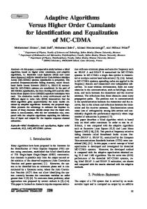
Figure 3-1. Surface plot CIM(X,0) in 2D sample space. (kernel width is 1) Figure 3-1 demonstrates the non-linear nature of the surface of the CIM, with N=2. Clearly the shape of L2 norm depends on the kernel function. Also the kernel bandwidth determines the extent L2 regions. As we will see later, these parameters play an important role in determining the quality of the final output.
24
CHAPTER 4 SELF-ORGANIZING MAPS WITH THE CORRENTROPY INDUCED METRIC As discussed in the previous chapter correntropy induces a non-linear metric in the input space called as Correntropy Induced Metric (CIM). Here we show that the CIM can be used as a similarity measure in the SOM to determine the winner and also to update the weight vectors. 4.1
On-line Mode
If v(n) is considered as the input vector of the random variable V at an instant n, then the best matching unit (BMU) can be obtained using the CIM as
r
= arg min CIM (v(n), w )N = arg min(κσ (0) − κσ (∥v(n) − w ∥)) s
s
(4–1)
=1
(4–2)
s
s
where r is consider as the BMU at instant n and σ is predetermined. According to Kohonen’s algorithm, if the CIM is used as the similarity measure then the local error that needs to be minimized to obtain an ordered mapping is given by
e (wr , v) =
M ∑ s =1
hrs (κσ (0) − κσ (∥v(n) − ws ∥))
(4–3)
For performing gradient descent over the local error for updating the weights, take the derivative of 4–3 with respect to ws and update the weights using the gradient. The update rule comes out to be
ws (n + 1) = ws (n) − η△ws
(4–4)
If the Gaussian function is used then the gradient is △ws
=
−hrs Gσ (∥v(n) − ws ∥)(v(n) − ws )
(4–5)
In case of Cauchy kernel, it is △ws
= −h (σ + ∥v(1n) − w ∥ ) (v(n) − w ) rs
2
s
25
2
s
(4–6)
The implicit σ term in 4–5 and 4–6 is combined with the learning rate η, a free parameter. When compared to the update rule obtained using the MSE (2–3), the gradient in both the cases have an additional scaling factor. This additional scaling factor, whose value is small when ∥v(n) − ws ∥ is large, in the updating rule points out the strong outliers rejection capability of the CIM. This property of the CIM is able to resolve one of the key problems associated with using MSE, i.e., over sampling the low probability regions of the input distribution. Since the weights are less influenced by the inputs in the low probability regions, the SOM with the CIM (SOM-CIM) can give a better magnification. It should be noted that since the influence of the outliers depends on the shape and extent of the L2-norm and L0-norm regions of the CIM, the magnification factor in turn is dependent on the type of the kernel and its bandwidth, σ. Another property of the CIM (with a Gaussian kernel), that influences the magnification factor, is the presence of higher order moments. According to Zador (1982) the order of the error directly influences the magnification factor of the mapping. Again, since the kernel bandwidth, σ, determines the influence of the higher order moments (refer to section 3.2 ) the choice of σ plays an important role in the formation of the final mapping. 4.2
Energy Function and Batch Mode
If the CIM is used for determining the winner and to update the weights, then according to Heskes (1999) an energy function over which the SOM can be adapted exist only when the winner is determined using the local error rather than just a metric. Hence, if the BMU is obtained by using
r
= arg min s
∑ t
hts CIM (v(n) − wt )
(4–7)
then the SOM-CIM is adapted by minimizing the following energy function.
e (W ) =
M ∑ s
hrs CIM (v(n) − ws )
26
(4–8)
In the batch mode, when a finite number of input samples are present the over all cost function becomes
ECIM (W ) =
N ∑ M ∑ n
s
hrs CIM (v(n) − ws )
(4–9)
Similar to the batch mode update rule obtained while using the MSE, we find the weight vectors at stationary point of the gradient of the above energy function, ECIM (W ). In case of the Gaussian kernel ∂ ECIM (W ) ∂ ws
=
⇒ ws
=
−
N ∑ n
∑N
hrs Gσ (v(n) − ws )(v(n) − ws ) = 0
hrs Gσ (v(n) − ws )v(n) n hrs Gσ (v(n) − ws )
n ∑ N
(4–10) (4–11)
The update here comes out to be the so called iterative fixed point update rule, indicating that the weights are updated iteratively and can not reach minima in one iteration, like it does with the MSE. And in case of the Cauchy kernel, the update rule is
ws =
∑N
hrs Cσ (v(n) − ws )v(n) n hrs Cσ (v(n) − ws )
n ∑ N
(4–12)
The scaling factor in the denominator and the numerator plays the similar role as described in the previous section 4.1. Figure 4-1 shows how the map evolves when the CIM is used to map 4000 samples of a uniform distribution between (0,1] on to a 7x7 rectangular grid. It shows the scatter plot of the weights at different epochs and the neighborhood relation between the nodes in the lattice are indicated by the lines. Initially, the weights are randomly chosen between (0,1] and the kernel bandwidth is kept constant at 0.1. A Gaussian neighborhood function, given by 4–13, is considered and its range is decreased with the number of epochs using 4–14. (
) ( r − s) hrs (n) = exp − 2σh (n) 2
27
(4–13)
A Random initial condition
B Epoch = 10
C Epoch = 30
D Epoch = 50
Figure 4-1. The figure shows the scatter plot of the weights along with the neighborhood nodes connected with the lines at various stages of the learning. σh (n) = σhi exp
(
n − θ ∗ σhi N
)
where r and s are node indexes, σh is the range of the neighborhood function, σhi value of σh , θ
(4–14)
= initial
= 0.3 and N = number of iterations/epochs.
In the first few epochs, when the neighborhood is large, all the nodes converge around the mean of the inputs and as the neighborhood decreases with the number of epochs, the nodes start to represent the structure of the data and minimizes the error. An another important point regrading the kernel bandwidth should be considered here. If the value of σ is small, then during the ’ordering phase’ (Haykin, 1998) of the
28
1
0.9
0.9
0.8
0.8
0.7
0.7
0.6
0.6 x2
x2
1
0.5
0.5
0.4
0.4
0.3
0.3
0.2
0.2
0.1
0.1
0
0
0.1
0.2
0.3
0.4
0.5 x1
0.6
0.7
0.8
0.9
0
1
0
0.1
A Constant kernel size
0.2
0.3
0.4
0.5 x1
0.6
0.7
0.8
0.9
1
B With kernel annealing
Figure 4-2. The scatter plot of the weights at convergence when the neighborhood is rapidly decreased. map the moment of the nodes is restricted because of the small L2 region. So, a slow annealing of the neighborhood function is required. To over come this, a large σ is considered initially, which ensures that the moment of the nodes is not restricted. It is gradually annealed during the ordering phase and kept constant at the desired value during the convergence phase. Figure 4-2 demonstrates this. When the kernel size is kept constant and the neighborhood function is decreased rapidly with θ
= 1 in 4–14, a
requirement for faster convergence, the final mapping is distorted. On the other hand, when the σ is annealed gradually from a large value to a small value, in this case 5 to 0.1, during the ordering phase and kept constant after that, the final mapping is much less distorted. Henceforth, this is the technique used to obtain all the results. In addition to this, it is interesting if we look back at the cost function (or local error) when the Gaussian kernel is used. It is reproduced here and is given by
eCIM (W ) =
=
∑
Mh s
∑
M ∑
rs
(1 − Gσ (w , v(n)))
hrs −
s
s
M ∑ s
29
hrs Gσ (ws , v(n))
(4–15)
(4–16)
The second term in the above equation can be considered as the estimate of the probability of the input using the sum of the Gaussian mixtures centered at the weights; with the neighborhood function considered equivalent to the posterior probability.
p(v(n)/W) ≈
∑ i
p(v(n)/wi )P (wi )
(4–17)
Hence, it can be said that this way of kerneling of the SOM is equivalent to estimating the input probability distribution (Yin, 2006). It can also be considered as the weighted Parzen density estimation (Babich and Camps, 1996) technique; with the neighborhood function acting as the strength associated with each weight vector. This reasserts the argument that the SOM-CIM can increase the magnification factor of the mapping to 1. 4.3
Results
4.3.1 Magnification Factor of the SOM-CIM As pointed out earlier, the use of the CIM does not allow the nodes to over sample the low probability regions of the input distribution as they do with the MSE. Also the presence of the higher order moments effect the final mapping but it is difficult to determine the exact effect the higher order moments have on the mapping here. Still, it can be expected that the magnification of the SOM can be improved using CIM. To verify this experimentally, we use a setup similar to that used by Ritter et al. (1992) to demonstrate the magnification of the SOM using the MSE. Here, a one dimensional input space is mapped onto a one dimensional map, i.e., a chain, with 50 nodes where the input is 100,000 instances drawn from the distribution
f (x ) = 2x . Then the relation between the weights and the node indexes are compared. A Gaussian neighborhood function, given by 4–13, is considered and its range is decreased with the number of iterations using 4–14 with θ
= 0.3.
If the magnification factor is ’1’, as in the case of optimal mapping, the relation between the weights and the nodes is ln(w )
= ln(r ). In case of the SOM with the 1 2
MSE (SOM-MSE) as the cost function, the magnification is proved to be 2/3 (Appendix.
30
0
−0.5
ln(w)
−1 Ideal Ideal with MSE
−1.5
σ = 0.03 σ = 0.5
−2
−2.5 −4
−3.5
−3
−2.5
−2 ln(r)
−1.5
−1
−0.5
0
Figure 4-3. The figure shows the plot between ln(r) and ln(w) for different values of σ. ’-’ indicates the ideal plot representing the relation between w and r when the magnification is 1 and ’...’ indicates the ideal plot representing the magnification of 2/3. ’-+-’ indicates relation obtained with SOM-CIM when σ = 0.03 and ’-x-’ indicates when σ = 0.5. A) and the the relation comes out to be ln(w )
= ln(r ). Figure 4-3 shows that when 3 5
smaller σ is considered for the SOM-CIM then a better magnification can be achieved. As the value of the σ increases the mapping resembles the one with the MSE as the cost function. This establishes the nature of the surface of CIM, as discussed in Section 3.2, that with the increase in the value of σ the surface tends to behave more like MSE. Actually, it can be said that with the change in the value of the σ the magnification factor of the SOM can vary between 2/3 to 1! But an analytical solution that can give a relation between the two is still elusive.
31
Table 4-1. The information content and the mean square quantization error for various value of σ in SOM-CIM and SOM with MSE is shown. Imax = 3.2189 Method Mean Square Entropy or Quantization Error Info Cont., I KSOM kernel Bandwidth, σ (. ∗ 10−3 ) 0.05 15.361 3.1301 Gaussian 0.1 5.724 3.2101 Kernel 0.2 5.082 3.1929 0.5 5.061 3.1833 0.8 5.046 3.1794 1.0 5.037 3.1750 1.5 5.045 3.1768 0.02 55.6635 3.1269 0.05 5.8907 3.2100 Cauchy 0.1 5.3305 3.2065 Kernel 0.2 5.1399 3.1923 0.5 5.1278 3.1816 1 5.0359 3.1725 1.5 5.0678 3.1789 MSE – 5.0420 3.1767 4.3.2 Maximum Entropy Mapping Optimal information transfer from the input distribution to the weights happen when the magnification factor is 1. Such a mapping should ensure that every node is active with equal probability, also called as equiprobabilistic mapping (Van Hulle, 2000). Since, the entropy is a measure that determines the amount of information content, we use Shannon’s entropy (4–18) of the weights to quantify this property.
I =−
M ∑
p(r)ln(p(r))
(4–18)
r
where p (r) is the probability of the node r to be the winner. Table 4-1 shows the change in I with the change in the value of the kernel bandwidth and the performance between the SOM-MSE and the SOM-CIM is compared. The mapping here is generated in the batch mode with the input having 5000 2-dimensional random samples generated from a linear distribution P (x ) ∝ 5x and mapped on to a 5x5 rectangular grid with σh
= 10 → 0.0045. 32
1 0.9 0.8 0.7 0.6 0.5 0.4 0.3 0.2 0.1 0
0
0.2
0.4
0.6
0.8
1
A Input scatter plot 1
1
0.9
0.9
0.8
0.8
0.7
0.7
0.6
0.6
0.5
0.5
0.4
0.4
0.3
0.3
0.2
0.2
0.1
0.1
0
0
0.2
0.4
0.6
0.8
0
1
B SOM - MSE
0
0.2
0.4
0.6
0.8
1
C SOM - CIM
Figure 4-4. The figures shows the input scatter plot and the mapping of the weights at the final convergence. (In case of SOM-CIM, the Gaussian kernel with σ = 0.1 is used.) The ’dots’ indicate the weight vectors and the lines indicate the connection between the nodes in the lattice space. From table 4-1, it is clear that as the value of the σ influences the quality of the mapping and figure 4-4 shows the weight distribution at the convergence. It is clear that, for large σ because of wider L2-norm region the mapping of the SOM-CIM behaves similar to that of the SOM-MSE. But as σ is decreased the nodes try to be equiprobabilitic indicating that they are not over sampling the low probability regions. But setting the value of σ too small again distorts the mapping. This is because of the restricted movement of the nodes; which leads to over sampling the high probability region. This underlines the importance the value of σ to obtain a good quality mapping.
33
3.5 3
Negative log−likelihood
2.5 2 1.5 1 0.5 0 −0.5
0
0.5
1 kernel bandwidth, σ
1.5
2
Figure 4-5. Negative log likelihood of the input versus the kernel bandwidth. The figure shows how the negative log likelihood of the inputs given the weights change with the change in the kernel bandwidth. Note that the negative value in the plot indicates that the model, the weights and the kernel bandwidth, is not appropriate to estimate the input distribution. It can also be observed how the type of the kernel also influences the mapping. The Gaussian and the Cauchy kernels give the best mapping at different values of σ, indicating that the shape of the L2 norm region for these two kernels are different. Moreover, since it is shown that the SOM-CIM is equivalent to density estimation, the negative log likelihood of the input given the weights is also observed when the Gaussian kernel is used. The negative log likelihood is given by
LL = −
N 1∑ log (p(v(n)/W, σ))
N
n
where p(v(n)/W, σ) =
1
M
M ∑ i
Gσ (v(n), wi )
(4–19) (4–20)
. The change in its value with the change in the kernel bandwidth is plotted in the figure 4-5. For an appropriate value of the kernel bandwidth, the likelihood of the estimating the input is high; where as for large values of σ it decreases considerably.
34
CHAPTER 5 ADAPTIVE KERNEL SELF ORGANIZING MAPS Now that the influence of the kernel bandwidth on the mapping is studied, one should understand the difficulty involved in setting the value of σ. Though it is understood from the theory of Correntropy (Liu et al., 2007) that the value of σ should be usually less than the variance of the input data, it is not clear how to set this value. Since the SOM-CIM can be considered as a density estimation procedure, certain rules of thumb, like the Silverman’s rule (Silverman, 1986) can be used. But it is observed that these results are suboptimal in many cases because of the Gaussian distribution assumption of the underlying data. It should also be noted that for equiprobabilistic modeling each node should adapt to the density of the inputs in it own vicinity and hence, should have its own unique bandwidth. In the following section we try to address this using an information theoretic divergence measure. 5.1 The Algorithm Clustering of the data is closely related to the density estimation. An optimal clustering should ensure that the input density can be estimated using the weight vectors. Several density estimation based clustering algorithms are proposed using information theoretic quantities like divergence, entropy, etc. There are also several clustering algorithms in the ITL literature like the Information Theoretic Vector Quantization (Lehn-Schioler et al., 2005), Vector Quantization using KL- Divergence (Hegde et al., 2004) and Principle of Relevant Information (Principe, 2010); where quantities like KL-Divergence, Cauchy-Schwartz Divergence and Entropy are estimated non-parametrically. As we have shown earlier, the SOM-CIM with the Gaussian kernel can also be considered as a density estimation procedure and hence, a density estimation based clustering algorithm. In each of these cases, the value of the kernel bandwidth plays an important role is the density estimation and should be set such that the divergence between the
35
true and the estimated pdf is as small as possible. Here we use the idea proposed by Erdogmus et al. (2006) of using the KullbackLeibler divergence (DKL ) to estimate the kernel bandwidth for density estimation and extend it to the clustering algorithms. As shown in section 3.1.2, the DKL (f ∥g ) can be estimated non-parametrically from the data using the Parzen window estimation. Here if f is the estimated pdf using the data and g is the estimated pdf using the weight vectors, then the DKL can be written as [
N ∑
DKL (f , g ) = Ev log (
i
]
Gσv (v − v(i )))
− Ev
[
M ∑
log (
j
]
Gσw (v − w(j )))
(5–1)
where σv is the kernel bandwidth for estimating the pdf using the input data and σw is the kernel bandwidth while using the weight vectors to estimate the pdf. Since we want to adapt the kernel bandwidth of the weight vector, minimizing DKL is equivalent to minimizing the second term in 5–1. Hence, the cost function for adapting the kernel bandwidth is
[
M ∑
J (σ) = −Ev log (
j
]
Gσw (v − w(j )))
(5–2)
This also called as the Shannon’s cross entropy. Now, the estimation of the pdf using the weight vector can be done using a single kernel bandwidth, homoscedastic, or with varying kernel bandwidth, heteroscedastic. We will consider each of these cases separately here. 5.1.1 Homoscedastic Estimation If the pdf is estimated using the weights with a single kernel bandwidth, given by
g=
M ∑ j
Gσw (v − w(j ))
(5–3)
then the estimation is called homoscedastic. In such a case only a single parameter needs to be adapted in 5–2. To adapt this parameter, gradient descent is performed over the cost function by taking the derivative of J (σ ) w.r.t σw . The gradient comes out to be
36
∂J ∂σw
=
−Ev
{ ∑M j
[
Gσw (v − w(j )) ∥v−σw(w j )∥ ∑M j Gσw (v − w(j ))
2
3
]} − σdw
To find an on-line version of the update rule, we use the stochastic gradient of the above update rule by replacing the expected value by the instantaneous value of the input. The final update rule comes out to be
= σw (n + 1) = △σw
where d
]} [ ∥v(n)−w(j )∥2 { ∑M − σdw 3 j Gσw (v(n) − w(j )) σw − ∑M j Gσw (v(n) − w(j )) σw (n) − η△σw
(5–5) (5–6)
= input dimensions and η is the learning rate.
This can be easily extended to the batch mode by taking the sample estimation of the expected value and finding the stationary point of the gradient. It comes out to a fixed point update rule, indicating that it requires a few epochs to reach a minima. The batch update rule is N ∑ 1 σw = Nd 2
n
∑M j
[
Gσw (v(n) − w(j )) ∥v(n) − w(j )∥2 ∑M j Gσw (v(n) − w(j ))
] (5–7)
It is clear from both on-line update rule 5–6 and batch update rule 5–7 that the value of σw is dependent on the variance of the error between the input and the weights localized by the Gaussian function. This localized variance converges such that the divergence between the estimated pdf and the true pdf of the underlying data is minimized. Hence, these kernels can be used to approximate the pdf density using the mixture of the Gaussian kernels centered at the weight vectors. We will get back to this density estimation technique in the later chapters. The performance of this algorithm is shown in the following experiment. Figure 5-1 shows the adaptation process of the σ where the input is a synthetic data consisting of 4 clusters centered at four points on a semicircle distorted with the Gaussian noise of 0.4 variance. The kernel bandwidth is adapted using the on-line update rule 5–6 by
37
1
3.5
0.9
3 2.5 2
0.7
feature 2
Kernel Bandwidth, σ
0.8
0.6
1.5 1
0.5
0.5
0.4
0.3
0
1
2
3
4
5 6 7 Number of Epochs
8
9
10
−0.5 −3
11
A
−2
−1
0 feature 1
1
2
3
B
Figure 5-1. Kernel adaptation in homoscedastic case.[A] The track of the σ value during the learning process in the homoscedastic case. [B] The scatter plot of the input and the weight vectors with the ring indicating the kernel bandwidth corresponding to the weight vectors. The kernel bandwidth approximates the local variance of the data. keeping the weight vectors constant at the centers of the clusters. It is observed that the kernel bandwidth, σ, convergence to 0.4041. This nearly equal to the local variance of the inputs, i.e., the variance of the Gaussian noise at each cluster center. However, the problem with the homoscedastic model is that if the window width is fixed across the entire sample, there is a tendency for spurious noise to appear in the tails of the estimates; if the estimates are smoothed sufficiently to deal with this, then essential detail in the main part of the distribution is masked. In the following section we try to address this by considering heteroscedastic model, where each node has unique a kernel bandwidth. 5.1.2 Heteroscedastic Estimation If the density is estimated using the weight vectors with varying kernel bandwidth, given by
g=
M ∑ j
Gσw (j ) (v − w(j ))
(5–8)
then the estimation is called heteroscedastic. In this case, the σ associated with each node should be adapted to the variance of the underlying input density surrounding 38
3.5
0.8 σ (1) σ (2) σ (3) σ (4)
0.75 0.7
3 2.5
0.65 2
0.6 0.55
1.5
0.5
1
0.45 0.5 0.4 0
0.35 0.3
1
2
3
4
5
6
7
8
9
10
−0.5 −3
11
−2
−1
A
0
1
2
3
B
Figure 5-2. Kernel adaptation in heteroscedastic case.[A] The plot shows the track of the σ values associated with their respective weights against the number of epochs. Initially, the kernel bandwidths are chosen randomly between (0,1] and are adapted using the on-line mode. [B] The scatter plot of the weights and the inputs with the rings indicating the kernel bandwidth associated with each node. the weight vector. We use the similar procedure as in the homoscedastic case, by substituting this in 5–1 and find the gradient w.r.t σw (j ). We get ∂J ∂σw (i )
[
{
Gσw (v − w(i )) ∥vσ−ww((i )i )∥ − σwd(i ) = −Ev ∑M j Gσw (j ) (v − w(j )) 2
3
]} (5–9)
Similar to the previous case, for on-line update rule we find the stochastic gradient and for batch mode update rule we replace the expected value with the sample estimation before finding the stationary point of the gradient. The update rules comes out to be: On-line Update rule:
△σw (n, i )
= σw (n + 1, i ) =
[ { i )∥ 2 d ]} Gσw (i ) (v(n) − w(i )) ∥v(nσ)w−(w( − 3 i) σw ( i ) − ∑M j Gσw (v(n) − w(j )) σw (n, i ) − η△σw (n, i )
Batch Mode Update rule:
39
(5–10) (5–11)
σw (i )2
= d1
∑N Gσw (i ) (v(n)−w(i )) ∑ n
[
∥v(n)−w(i )∥2
]
M Gσ (j ) (v(n)−w(j )) j w Gσw (i ) (v(n)−w(i )) n ∑Mj Gσw (j ) (v(n)−w(j ))
∑N
(5–12)
Figure 5-2 shows the kernel bandwidth adaptation for a similar setup as described for the homoscedastic case (5.1.1). Initially, the kernel bandwidths are considered randomly between (0,1] and are adapted using the on-line learning rule (5–11) while keeping the weight vectors constant at the centers of the clusters. The kernel bandwidth tracks associated with each node are shown and the σ associated with each node again converged to the local variance of the data. 5.2
SOM-CIM with Adaptive Kernels
It is easy to incorporate the above mentioned two adaptive kernel algorithms in the SOM-CIM. Since the value of the kernel bandwidth adapts to the input density local to the position of the weights, the weights are first updated followed by the kernel bandwidth. This ensures that the kernel bandwidth adapts to the present position of the weights and hence, better density estimation. The adaptive kernel SOM-CIM in case of homoscedastic components can be summarized as: •
The winner is selected using the local error as
r •
= arg min
M ∑
s
hst (Gσ(n) (0) − Gσ(n) (∥v(n) − wt ∥))
(5–13)
t
The weights and then the kernel bandwidth are updated as
= w (n + 1) = △ws
s
△σ (n)
=
σ (n + 1)
=
−hrs Gσ(n) (∥v(n) − ws ∥)
ws (n) − η△ws
(v(n) − w ) σ (n ) s
3
(5–14) (5–15)
{ ∑M G (v(n) − w (n + 1)[ ∥v(n)−wj (n+1)∥2 − d ] } j j σ( n ) σ( n ) 3 σ( n ) − (5–16) ∑M G ( v ( n ) − w ( n + 1) j σ n ) j ( σ (n) − ησ △σ (n) (5–17)
40
•
In the batch mode, the weights and the kernel bandwidth are updated as
ws
+
σ+
∑N
hrs Gσ (v(n) − ws )v(n) n hrs Gσ (v(n) − ws ) N ∑M G (v(n) − w )[∥v(n) − w ∥2 ] ∑ 1 j j j σ = Nd ∑M j Gσ (v(n) − wj ) n
=
n ∑ N
(5–18) (5–19)
In case of heteroscedastic kernels, the same update rules apply for the weights but with σ specified for each node; while the kernel bandwidths are updated as On-line mode: △σi (n)
= σi (n + 1) =
[ ] 2 { Gσi (n) (v(n) − wi (n + 1)) ∥v(n)−σiw(ni ()n3+1)∥ − σi d(n) } − ∑M j Gσj (n) (v(n) − wj (n + 1) σi (n) − ησ △σi (n)
Batch mode:
σi+
= d1
∑N Gσi (v(n)−wi ) ∑ n
[
∥v(n)−wi ∥2
(5–20) (5–21)
]
M Gσ (v(n)−wj ) j Gσw (i ) (v(n)−w(i )) n ∑Mj Gσw (j ) (v(n)−w(j ))
∑N
(5–22)
But it is observed that when the input has a high density part, compared to the rest of the distribution, the kernel bandwidth of the weights representing these parts shrinks too small to give any sensible similarity measure and makes the system unstable. To counter this, a scaling factor ρ can be introduced as △σi (n)
=
[ ] 2 { Gσi (n) (v(n) − wi (n + 1)) ∥v(n)−σiw(ni ()n3+1)∥ − σi d(n) } − ∑M j Gσj (n) (v(n) − wj (n + 1)
(5–23)
This ensures that the value of the σ does not go too low. But at the same time it inadvertently increases the kernel bandwidth of the rest of the nodes and might result in a suboptimal solution. The experiment similar to that in section 4.3.1 clearly demonstrates this. 100,000 samples from the distribution f (x )
= 2x are mapped on
to a 1D chain of 50 nodes in on-line mode and the relation between the weights and the node indexes is observed. Figure 5-3 shows the results obtained. Clearly in case of the homoscedastic case the mapping converge to the ideal mapping. But in case of
41
0.7
0.6
0.6
0.5
0.5 kernel bandiwdth, σ
Kernel Bandwidthm; σ
0.7
0.4 0.3
0.4
0.3
0.2
0.2
0.1
0.1
0
0
2
4 6 Number of Iterations
8
0
10
0
2
4 6 Number of Iterations
4
x 10
A
8
10 4
x 10
B 0
0 −0.5 −0.5 −1
ln w
ln(w)
−1
Ideal Ideal with MSE Adaptive kernel
−1.5
−2
−2.5
−2
−2.5 −4
−1.5
−3.5
−3
−2.5
−2 ln r
−1.5
−1
−0.5
−3 −4
0
−3.5
−3
C
−2.5
−2 ln(r)
−1.5
−1
−0.5
0
D
Figure 5-3. Magnification of the map in homoscedastic and heteroscedastic cases.The Figures [A] and [B] shows the tracks of the kernel bandwidth in case of homoscedastic and heteroscedastic kernels, respectively. Figures [C] and [D] shows the plot between ln(r) and ln(w). ’- -’ indicates the ideal plot representing the relation between w and r when the magnification is 1 and ’...’ indicates the ideal plot representing the magnification of 2/3. ’-+-’ indicates relation obtained with adaptive kernels SOM-CIM in homoscedastic and heteroscedastic cases, respectively. Refer text for explanation. the heteroscedastic kernels it is observed the the system is unstable for ρ
= 1. Here
to obtain a stable result ρ is set to 0.7. This stabilizes the mapping by not allowing the kernel bandwidth to shrink too small. But it clearly increases the kernel bandwidth of the nodes in low probability region and hence, the distortion in 5-3D. It is also interesting to see the changes in the kernel bandwidth while adapting in the Figure 5-3A and Figure 5-3B. Initially, all the kernels converge to the same
42
Table 5-1. The information content and the mean square quantization error for homoscedastic and heteroscedastic cases in SOM-CIM. Imax = 3.2189 Method Mean Square Entropy or Quantization Error Info Cont., I Homoscedastic kernels 5.8725 ∗ 10−3 3.2095 −3 Heteroscedastic kernels (ρ = 0.5) 6.1179 ∗ 10 3.1970 Heteroscedastic kernels (ρ = 1) 15.268 ∗ 10−3 2.700 1 −3 Constant kernel , σ = 0.1 5.7240 ∗ 10 3.2101 −3 MSE 5.0420 ∗ 10 3.1767 1
0.8
0.9
0.7
0.8 0.6 Kernel bandwidth, σ
0.7
feature 2
0.6 0.5 0.4
0.5 0.4 0.3
0.3 0.2 0.2 0.1
0.1 0
0
0.2
0.4
0.6
0.8
0
1
0
10
feature 1
20 30 Number of Epochs
40
50
Figure 5-4. Mapping of the SOM-CIM with heteroscedastic kernels and ρ = 1. bandwidth as the nodes are concentrated at the center and as map changes from the ordering phase to the convergence the kernel bandwidths adapt to the local variance of each node. This kind of adaptation ensures that the problem of slow annealing of the neighborhood function, discussed in section 4.1, can be resolved by having relatively large bandwidth at the beginning, allowing the free movement of the nodes during ordering phase. As the adaptive kernel algorithm is able to map the nodes near to the optimal mapping, it is expected to transfer more information about the input density to the
1
The best result from Table 4-1 is reproduced for comparison.
43
1 0.9
0.8
0.8
0.7
0.7
0.6
0.6 feature 2
feature 2
1 0.9
0.5
0.5
0.4
0.4
0.3
0.3
0.2
0.2
0.1
0.1
0
0
0.2
0.4
0.6
0.8
0
1
0
0.2
0.4
0.6
feature 1
feature 1
A
B
0.8
1
Figure 5-5. The scatter plot of the weights at convergence in case of homoscedastic and heteroscedastic kernels. [A] The scatter plot of weights in case of homoscedastic kernels. [B] The scatter plot of weights in case of heteroscedastic case. The lines indicate the neighborhood in the lattice space. Clearly, the heteroscedastic kernels with ρ = 0.5 over sample the low probability regions when compared with the homoscedastic case. weights. Results obtained for the experiment similar to the one in section 4.3.2, where the inputs are 5000 samples from the 2 dimensional distribution with pdf f (x )
= 5x
mapped on to a 5x5 rectangular grid, are shown in Table 5-1. With the homoscedastic kernels, the kernel bandwidth converged to 0.0924, which is close to the value that is obtained as the best result in Table 4-1 (σ
= 0.1) and at the same time is able to
transfer more information to the weights. But in the heteroscedastic case the system is unstable with ρ
= 1 and fails to unfold (5-4), concentrating more on the high probability
regions. On the other hand, when ρ is set to 0.5, the resulting map does not provide a good output because of the large σ values. Figure 5-5 clearly demonstrates this. When ρ
= 0.5, it clearly over samples the low probability regions because of the large kernel
bandwidths of the nodes representing them.
44
CHAPTER 6 APPLICATIONS Now that we saw how the SOM can be adapted using the CIM, in this chapter we try to use the SOM-CIM in few of the applications of the SOM; like density estimation, clustering and principal curves, and show that how it can improve the performance. 6.1
Density Estimation
Clustering and density estimation are closely related and one is ofter used to find the other, i.e., density estimation is used find the clusters (Azzalini and Torelli, 2007) and clustering is used to find the density estimation (Van Hulle, 2000). As we have shown earlier SOM-CIM is equivalent to a density estimation procedure and with the adaptive kernels it should be able to effectively reproduce the input density using the Parzen non-parametric density estimation procedure (Parzen, 1962). Here we try to estimate a 2 dimensional Laplacian density function shown in Figure 6-1A. The choice of the Laplacian distribution is appropriate to compare these methods because it is heavy tail distribution and hence, is difficult to estimate without the proper choice of the kernel bandwidth. Figure 6-1 and Table 6-1 shows the results obtained when different methods are used to estimate the input density. Here 4000 samples of a 2 dimensional Laplacian distribution are mapped on to a 10x10 rectangular grid. The neighborhood function is given by 4–13 and is annealed using 4–14 with θ
= 0.3 and σhi = 20. When the
SOM-MSE is used the kernel bandwidth is estimated using Silverman’s rule (Silverman, 1986): σ
= 1.06σf N −
5
(6–1)
where σf is the variance of the input and N is the number of input samples. Figure 6-1B clearly demonstrates that this procedure not able to able to produce a good result because of the large number of bumps in the low probability regions. This is because
45
0.25 0.25 0.2 0.2 0.15 0.15 0.1
0.1
0.05
0.05
0 10
0 10 5
6
5
4
0
2
0
0
−5
−2 −10
−5
−4
−10
−6
A True density function
−6
−4
−2
0
2
4
6
B SOM with MSE
0.25
0.25
0.2
0.2
0.15
0.15
0.1
0.1
0.05
0.05
0 −10
0 10 −5 0 5 10
−6
−4
−2
0
2
4
5
6
−6 −4
0
−2 0
−5
2 −10
C SOM-CIM with homoscedastic kernels
4 6
D SOM-CIM with heteroscedastic kernels
Figure 6-1. Results of the Density estimation using SOM. [A] A 2 dimensional Laplacian density function. [B] The estimated density using SOM with MSE. The kernel bandwidth is obtain using the Silverman’s rule. [C] The estimated density using SOM-CIM with homoscedastic kernels. [D] The estimated density using SOM-CIM with heteroscedastic kernels. of the oversampling of the low probability regions when MSE is used, as discussed in section 2.3. On the other hand, the use of the SOM-CIM, with both homoscedastic and heteroscedastic kernels, is able to reduce the oversampling of the low probability regions. But in case of homoscedastic kernels, because of the constant bandwidth of the kernels for all the nodes, the estimation of the tail of the density is still noisy and is unable to clearly demonstrate the characteristics of the main lobe of the density properly.
46
Table 6-1. Comparison between various methods as density estimators. MSE and KLD are the mean square error and KL-Divergence, respectively, between the true and the estimated densities. Method MSE (. ∗ 10−4 ) KLD SOM with MSE 2.0854 308.4163 SOM-CIM, homoscedastic 2.0189 128.6758 heteroscedastic(ρ = 0.8) 3.1432 12.6948 This is resolved when the heteroscedastic kernels are used. Because of the varying kernel bandwidth, it is able to smooth out the tail of the density while still retaining the characteristics of the main lobe and hence, able to reduce the divergence between the true and estimated densities. 6.2
Principal Surfaces and Clustering
6.2.1 Principal Surfaces Topology preservation maps can be interpreted as an approximation procedure for the computation of principal curves, surfaces or higher-dimensional principal manifolds (Ritter et al., 1992). The approximation consists in the discretization of the function
f
defining the manifold. The discretization is implemented by means of a lattice A
of corresponding dimension, where each weight vector indicates the position of a surface point in the embedding space V . Intuitively, these surface points, and hence the principal curve, are expected to pass right through the middle of their defining density distribution. This definition of principal surfaces in 1 dimensional case, and can be generalized to high dimensional principal manifold as (Ritter et al., 1992): Let f (s ) be a surface in the vector space V , i.e, dim(f ) − dim(V ) − 1, and let df (v) be the shortest distance of a point v ∈ V to the surface f . f is a principal surface correspondong to the the density distribution P (v) in V , if the “mean squared distance” ∫
Df =
df2 (v)P (v)d L v
is extremal with respect to local variation of the surface.
47
4
4
2
2
0
0
−2
−2
−4
−4
−6
−6
−8 −4
−2
0
2
−8 −4
4
−2
A With MSE
0
2
4
B 10 Epochs 4
4 2 2 0 0 −2 −2 −4
−4
−6
−6
−8 −5
0
−8 −4
5
C 20 Epochs
−2
0
2
4
D 50 Epochs
Figure 6-2. Clustering of the two-crescent dataset in the presence of out lier noise. [A] The mapping at the convergence of SOM with MSE. [B] - [D] The scatter plot of the weights with the kernel bandwidth at different epochs during learning. But the use of the MSE as the criteria for the goodness of the principal surfaces, makes it weakly defined because only the second order moments are used and also the distortion in the mapping when outliers are present. Figure 6-2A shows this when the two crescent data is slightly distorted by introducing some outliers. On the other hand, if the principal surface is adapted in the correntropy induced metric sense, then the effect of the outliers can be eliminated and gives a better approximation of the principal surfaces. Figure 6-2 illustrates this in case of the SOM-CIM with homoscedastic kernels,
48
2.5
2.5
2
2
1.5
1.5
1
1
0.5
0.5
0
0
−0.5
−0.5
−1
−1
−1.5
−1.5
−2 −2
−1.5
−1
−0.5
0
0.5
1
1.5
−2 −2
2
−1.5
−1
−0.5
0
0.5
1
1.5
2
Figure 6-3. The scatter plot of the weights showing the dead units when CIM and MSE are used to map the SOM. [A] The boxed dots indicate the dead units mapped when MSE is used. [B] Mapping when CIM with σ = 0.5 is used in the SOM. There are no dead units in this case. where the kernel bandwidth adapts such that the outliers does not have significant effect the final mapping throughout the learning. 6.2.2 Avoiding Dead Units Another problem with the SOM is that it can yield nodes that are never active, called as dead units. These units will not sufficiently contribute to the minimization of the overall distortion of the map and, hence, this will result in a less optimal usage of the map’s resources (Van Hulle, 2000). This is acute when there are clusters of data that are far apart in the input space. The presence of the dead units can also be attributed to the MSE based cost function which pushes the nodes into these regions. Figure 6-3A indicates this where the input contains three nodes, each is skewed by 500 samples of a 2 dimensional Gaussian noise with variance equal to 0.25. On the other hand, when CIM is used, as indicated in section 4.3.2, the mapping tries to be equiprobabilistic and hence, avoids dead units (Figure 6-3B).
49
Table 6-2. Number of dead units yielded for different datasets when MSE and CIM are used for mapping. Each entry is an average over 30 runs. Dataset Method Dead Units MSE (10−2 ) Artificial MSE 4 1.3877 CIM, σ = 0.2147 0 8.4458 Iris MSE 5.6 5.939 CIM, σ = 0.5 1 8.023 Blood Transfusion MSE 0 0.7168 CIM, σ = 0.2 0 0.8163 Table 6-2 show the results obtained over three different datasets mapped on to 10x5 hexagonal grid. The artificial dataset is the same as the one described above. The Iris and Blood transfusion datasets are obtained from the UC Irvine repository. The Iris dataset contains 3 classes of 50 instances each, where each class refers to a type of iris plant. Here, one class is linearly separable from the other 2; the latter are not linearly separable from each other, and each instance has 4 features. It is observed that the dead units appear in between the two linearly separable cases. The blood transfusion dataset (normalized to be between [0,1] before mapping) contains 2 classes with 24% positive and 76% negative instances. Though there are no dead units in this case, as we will show later, this kind of mapping neglects the outliers and hence able to give a better visualization of the data. An other important observation is, the adaptive kernel algorithms are unable to give a good result for both Iris and Blood Transfusion datasets. The reason for this is the inherent nature of the Parzen density estimation, which is the center piece for this algorithm. As the number of dimensions increase the number of input samples required by the Parzen density estimation for proper density estimation increases exponentially. Because of the limited amount of data in these datasets the algorithm failed to adapt the kernel bandwidth.
50
Figure 6-4. The U-matrix obtained for the artificial dataset that contains three clusters. [A] U-matrix obtained when the SOM is trained with MSE and the euclidian distance is used to create the matrix. [B] U-matrix obtained when the CIM is used to train the SOM and to create the matrix. 6.3 Data Visualization Visualizing high dimensional data in low dimensional grid is one of the important applications of SOM. Since the topography can be preserved on to the grid, visualizing the grid can give a rough idea about the structure of the data distribution and, in turn, an idea about the number of clusters without any apriori information. The popular SOM visualization tool is the U-matrix, where the distance between the a node and all its neighbors is represented in a gray scale image. If the euclidean distance is used to construct the matrix, then the distance between the closely spaced clusters is over shadowed by the far away clusters, making it difficult to detect them. On the other hand, because of the non-linear nature of the CIM and saturation region beyond certain point (determined by the value of σ), the closely spaced clusters can be detected if the U-matrix is constructed using CIM. Figure 6-4 shows the results obtained when the MSE and the CIM are used to train the SOM and to construct the U-matrix. The SOM here is a 10x5 hexagonal grid and
51
A
B
C
D
Figure 6-5. TThe U-matrix obtained for the Iris and blood transfusion datasets. [A] and [C] show the U-matrix for the Iris and Blood transfusion datasets, respectively, when the SOM is trained with MSE and the euclidian distance is used to create the matrix. [B] and [D] show their corresponding U-matrix obtained when the CIM is used to train the SOM and to create the matrix.
52
the input is a 2 dimensional artificial dataset containing 3 clusters; one cluster is farther away from the other two (6-3), each made up of 500 instances of the Gaussian noise with variance 0.25. Clearly, the boundaries are not crisp when the MSE is used. This is because of the dead units the SOM yields when the MSE is used. On the other hand, the U-matrix obtained when the SOM-CIM is used is able to give a crisp boundaries. The problem of viewing closely space clusters when there are other outliers or faraway clusters becomes even more difficult. Figure 6-5 illustrates this is the case of the Iris dataset and the Blood transfusion dataset. The Iris dataset has three clusters where only one cluster is linearly separable from the other two. When the U-matrix is created using the MSE, only the linearly separable cluster is distinguishable from the other two. Where as, the U-matrix created using the CIM is able to show the three clusters (though not with crisp boundaries). The reason for this is not only because of avoiding the dead units but also because of the non-linear norm of the CIM. If the distance between the nodes that are closely space (in euclidian sense) is evaluated using the CIM, then this is not over shadowed by the distance evaluated using the CIM between the nodes thats are far apart because of the saturation of the CIM norm. The blood transfusion dataset has two clusters and expected to have large number of outliers. The quality of the U-matrix is not discussed and is left to the readers.
53
CHAPTER 7 CONCLUSION The use of the kernel Hilbert spaces by Vapnik (1995) has spurred the use of the kernel methods is several field. This idea is also used in the self organizing maps previously by Lau et al. (2006),Andras (2002), MacDonald (2000), etc. In all these cases the use of the kernel trick is viewed in context of the pattern classification and the increase in the performance is attributed to the assumption that the classes tend to be linearly separable when mapped into higher dimensions. On the other hand, the use of the correntropy induced metric gives an idea about effect the kernelization has in the input space and hence, is able to give an idea about how the final output of the mapping is effected by the choice of the kernel and kernel bandwidth. As indicated, the choice of the kernel bandwidth dictates the magnification of the mapping. For example, larger bandwidth adapt the SOM-CIM to minimize the quantization error because of the large L2-norm induced, where as smaller bandwidth might result in a map that concentrates more on the high probability parts; and hence, distorting the mapping. Also, as previously discussed, the advantage of using the CIM lies in its strong outlier’s rejection capability and the presence of higher order moments. Both these properties are useful when the input distribution is non-uniform and hence, the SOM-CIM can outperform the SOM only when the data in non-uniformly distributed (true for many practical cases). The proposed adaptive kernel algorithm based on the KL-divergence is able to adapt the bandwidth nearly to the optimal solution. But it is observed that the algorithm is unstable in the heteroscedastic case and an additional free parameter ρ needs to be specified. In spite of that, the final mapping is still less sensitive to the value of ρ than the value of σ and is also able to give a heteroscedastic alternative. Another point that needs to be discussed is the extension of the use of the CIM in other clustering algorithms like neural-gas, elastic nets, soft-topographic vector
54
quantization 1 , etc. The similarity measure used in the ranking of the weight vectors in the neural gas algorithm can be replaced by the CIM and a similar procedure can be applied to adapt the the network. This is also expected to improve the performance of the network in terms of the magnification factor. Finally, though the dependence of the magnification factor on the kernel bandwidth is shown experimentally, the analytical analysis is still illusive. The future work should concentrate on the finding the relation between the magnification factor and the kernel bandwidth; which in turn depends on the variance of the data. Also the use of multivariate kernels might be important when the SOM-CIM is used for density estimation and it also needs to be studied. The proposed adaptive kernel algorithm can also be extended to the multivariate kernels using the idea proposed by Erdogmus et al. (2006) but will lead to a larger computational complexity. An effective, less computationally expensive algorithm to adapt the kernel bandwidth is necessary.
1
This is discussed in Appendix B 55
APPENDIX A MAGNIFICATION FACTOR OF THE SOM WITH MSE The quantitative analysis of the magnification factor of the SOM with the MSE as the cost function is shown here. Detailed analysis of this can be found at (Ritter et al., 1992). The along as the neighborhood function hrs is non-zero, w (r, t ) undergoes a non-zero change at each time step. This transition of the weights from w to w ^ can be formally by the transformation
w = T (w ^ , v, ϵ)
(A–1)
where ϵ is the learning rate. Explicitly, the transition in A–1 can be written as
ws = w ^ s + ϵhrs (v − w ^ s ), ∀s
(A–2)
. Since the input v occurs only with the probability P (v), the probability Q (w, w ^ ) of the transition from the state w to w ^ can be written as
Q (w, w^ ) =
∫
δ (w − T (w ^ , v, ϵ))P (v)d v
(A–3)
In the equilibrium condition, the necessary and sufficient condition is that the transition probability to be zero. This implies
∫ ⇒
Q (w, w^ ) = 0 ϵhrs (v − ws )P (v)d v
= = 0 ∀s
(A–4)
A maximally ordered map, defined as a map that is fully unfolded without any ’twists’ or ’kinks’, is assumed which leads to the validity of the following assumptions in the continuum case •
It is assumed that for a sufficiently large systems wr is a function of that varies slowly from lattice point to lattice point so that its replacement by a function w(r) on a continuum of r-values is justified.
•
We assume that w(r) is one-to-one.
56
Also the the neighborhood function with a steep maximum at r = s that satisfies ∫ ∫
hrs (r − s)d r = 0
h(r − s)(ri − si )(rj − sj )d r =
δij σh2 , ∀i , j
= 1, 2, ..., d
(A–5)
where d is the dimensionality of the lattice, which is assumed same as the dimensionality of the input space V and σh is the neighborhood range of the Gaussian neighborhood function used. Due to the continuum approximation where it is assumed that there are infinite number of nodes, at the equilibrium, the quantity ∥v − wr ∥ vanishes since each sample
v in the input space has a corresponding to an r for which v
= w . So, we can replace v r
in A–4 with wr . Also, by changing the variable of integration to s instead of w, the A–4 becomes
∫
hrs (wr − ws )P (wr )J (wr )d s = 0
Here
J (wr ) = |
dv s
|
is the absolute value of the Jacobian of the map ϕw
� (r) intergration variable and P
(A–6)
(A–7)
: v → w. With q = r − s as a new
= P (w(r)) the expansion of
A–6 in the powers of q yields
(with implicit summation qi ∂i is to be summed over all i ) ∫
1 2 .(P� + ∂k P� + ...)(J + ql ∂l J + ...)d q ∫ = h (qi ∂i wP� J + qi qk ∂i w∂k P� J +qi ql ∂i w∂l J P� + ...)d q ∫ ( ) = h d q. (∂i w)∂j (P� J ) + 21 P� J .∂i ∂j w (s) + O (σh ) [ ] = σh (∂i w)∂j (P� J ) + 12 P� J .∂i w (r) + O (σh )
0 =
hq0 (qi ∂i w + qi qj ∂i ∂j w + ...).
(A–8)
q0
4
q0
2
2
57
4
(A–9)
where the condition about the neighborhood function in A–5 are used. The necessary and sufficient condition for A–9 to hold for small σ is ∑ i
( ∂i w
Substituting the Jacobian matrix Jij
� ∂i P
∂i J
+ J P�
)
∑ = − 21 ∂i w 2
(A–10)
i
= ∂j wi (r) and △ = ∑i ∂i , the condition becomes 2
1 2
� .J) = − △w J.ln(P For a one-dimensional case we obtain J
(A–11)
= J = dw /dr and △w = d w /dr 2
2
with w and r
as scalars. Using this the differential equation A–10 can be solved. Rewriting the above equation by substituting these values, we get (
(
dw 1 d P� dw + � dr P dr dr from which we can obtain
)− 1
)
d 2w 1 d 2w = − dr 2 2 dr 2 (
d � 3 d dw lnP = − ln dr 2 dr dr
Since ϕw (w(r))
(A–12)
) (A–13)
= r holds, the local magnification factor M of ϕw can be defined by M = 1/J . For the one-dimensional case M = (dw /dr )− and we obtain as a relation 1
between input stimulus distribution and the lattice representation
M (v ) = J −1 =
dr dw
∝ P (v )2/3
(A–14)
Hence, the local magnification factor M(v) is dependent on the probability density P (v ) according to a power law with factor 2/3. The condition that need to be solved for obtaining the magnification factor of the SOM-CIM, at the equilibrium condition, is ∫
hrs Gσ (v − ws )(wr − ws )P (v)d v = 0
This is left for the future work.
58
(A–15)
APPENDIX B SOFT TOPOGRAPHIC VECTOR QUANTIZATION USING CIM Graepel et al. (1997) has used deterministic annealing (Rose, 1998) in topographic preserving vector quantization. The idea is to reduce the free energy of the clustering nodes while maintaining the topology of the nodes in the lattice space. The algorithm can be described in the following sections. B.1
SOM and Free Energy
With the local error in 2–2 deciding the winner, the quantization error over the entire dataset is given by
Fquant (P , W ) =
∑∑
prn
∑
hrs D (vn , ws )
(B–1)
n r s n where pr is the posterior probability that the node r is the winner when vn is considered
and the entropy term which determines the probability of the nodes to occur is given by
Fent (P ) =
∑∑ n
r
prn log
prn qr
(B–2)
where qr = prior probability of the nodes. Using the B–1 and B–2, the free energy of the function can be written as
F (P , W ) = β Fquant (P , W ) + Fent (P )
(B–3)
where β is called the inverse temperature, larger the β lesser the influence of the entropy (Heskes, 2001). B.2 Expectation Maximization As proved by Neal and Hinton (1998) that the (local) minimum of the free energy corresponds to the (local) minimum error of the self organizing maps, expectation maximization can be used to find the optimal solution (Heskes, 2001; Neal and Hinton, 1998) of the weights and their corresponding posteriors. The expectation step corresponds to finding the posteriors, prn , that minimizes the ∑ F (P , W ). By using a Lagrange multiplier with the condition that r prn = 1, the optimal
59
1
1
0.9
0.9
0.8
0.8
0.7
0.7
0.6
0.6
0.5
0.5
0.4
0.4
0.3
0.3
0.2
0.2
0.1
0.1
0
0
0.2
0.4
Aβ
0.6
0.8
0
1
0.9
0.9
0.8
0.8
0.7
0.7
0.6
0.6
0.5
0.5
0.4
0.4
0.3
0.3
0.2
0.2
0.1
0.1 0.2
0.4
Cβ
0.6
0.4
Bβ 1
0
0.2
= 0.01
1
0
0
0.8
0
1
0
0.2
0.4
Dβ
= 250
0.6
0.8
1
0.8
1
= 100
0.6
= 500
Figure B-1. The unfolding of the SSOM mapping when the CIM is used as the similarity measure. The snapshots are taken at intermediate point during the unfolding of the mapping at different values of β. The dataset considered here is a uniform distribution of 1000 points within a unit square. The neighborhood function is fixed at σh = 0.5 . posteriors can be obtained and it comes out to be
prn
∑
t hrt D (vn , wt )) ∑ = ∑qrqexpexp(−β (−β t hst D (vn , wt)) s s
(B–4)
This update rule does not depend on the distance measure and hence, would be same while using both the MSE and CIM measures.
60
Whereas the maximization step changes with the similarity measure. With MSE By finding the derivative of Eq. 5 w.r.t weights, ws , and equating it to zero, we get the updation rule as in Eq. 9.
ws (i ) =
∑ ∑ n pr hrs x µ (i ) n∑ r∑ n n
r pr hrs
(B–5)
With CIM While using the CIM, the fixed point update rule is
ws (i ) =
∑ ∑ n n n ∑ r pr hrs Gσ (vn − ws )v (i ) ∑ n n r pr hrs Gσ (vn − ws )
(B–6)
With hrs → δ, STVQ acts as a traditional SOM with soft membership function (Graepel et al., 1997). Figure B-1 shows the evolution of the soft SOM (SSOM) when CIM with σ
= 0.5 is used. Since the use of deterministic annealing is to avoid the local
minima of the cost function, the discussion about the magnification of the mapping still holds here. It is expected that the use of the CIM here plays a similar role as in the case of the SOM-CIM.
61
REFERENCES Andras, P. “Kernel-Kohonen networks.” International Journal of Neural Systems 12 (2002): 117–135. Azzalini, Adelchi and Torelli, Nicola. “Clustering via nonparametric density estimation.” Statistics and Computing 17 (2007): 71–80. Babich, Gregory A. and Camps, Octavia I. “Weighted Parzen Windows for Pattern Classification.” IEEE Transactions on Pattern Analysis and Machine Intelligence 18 (1996): 567–570. Bauer, H. U. and Der, R. “Controlling the magnification factor of self-organizing feature maps.” Neural Comput. 8 (1996).4: 757–771. Bell, Anthony J. and Sejnowski, Terrence J. “An information-maximization approach to blind separation and blind deconvolution.” Neural Comput. 7 (1995).6: 1129–1159. Claussen, Jens Christian. “Winner-Relaxing Self-Organizing Maps.” Neural Comput. 17 (2005).5: 996–1009. Deniz Erdogmus, Jose C. Principe. “Generalized Information Potential Criterion for Adaptive System Training,.” Trans. on Neural Networks 12 (2002).5: 1035–1044. Erdogmus, Deniz, Jenssen, Robert, Rao, Yadunandana N., and C.Principe, Jos. “Gaussianization: An Efficient Multivariate Density Estimation Technique for Statistical Signal Processing.” The Journal of VLSI Signal Processing 45 (2006): 67 –83. Erwin, E., Obermayer, K., and Schulten, K. “Self-Organizing Maps: Ordering, Convergence Properties and Energy Functions.” Biological Cybernetics 67 (1992): 47–55. Graepel, T. “Self-organizing maps: Generalizations and new optimization techniques.” Neurocomputing 21 (1998).1-3: 173–190. Graepel, Thore, Burger, Matthias, and Obermayer, Klaus. “Deterministic Annealing for Topographic Vector Quantization and Self-Organizing Maps.” Proceedings of the Workshop on Self-Organising Maps, volume 7 of Proceedings in Artificial Intelligence. Infix, 1997, 345–350. Haykin, Simon. Neural Networks: A Comprehensive Foundation (2nd Edition). Prentice Hall, 1998, 2 ed. Hegde, A., Erdogmus, D., Lehn-Schiøler, T., Rao, Y., and Principe, J. “Vector-Quantization by density matching in the minimum Kullback-Leibler divergence sense.” IEEE International Conference on Neural Networks - Conference Proceedings. vol. 1. 2004, 105–109.
62
Heskes, T. “Self-organizing maps, vector quantization, and mixture modeling.” Neural Networks, IEEE Transactions on 12 (2001).6: 1299–1305. Heskes, Tom. Energy function for self-organizing maps. Amsterdam: Elsevierl, 1999. Kohonen, Teuvo. “Self-organized formation of topologically correct feature maps.” Biological Cybernetics 43 (1982): 59 – 69. ———. Self-Organizing Maps (2nd ed)(Springer Series in Information Sciences, 30). Springer, 1997, 2nd ed. Lau, K., Yin, H., and Hubbard, S. “Kernel self-organising maps for classification.” Neurocomputing 69 (2006).16-18: 2033–2040. Lehn-Schioler, Tue, Hegde, Anant, Erdogmus, Deniz, and Principe, Jose. “Vector quantization using information theoretic concepts.” Natural Computing 4 (2005).1: 39–51. Linsker, Ralph. “How to generate ordered maps by maximizing the mutual information between input and output signals.” Neural Comput. 1 (1989).3: 402–411. Liu, Weifeng, Pokharel, Puskal P., and Principe, Jose C. “Correntropy: Properties and Applications in Non-Gaussian Signal Processing.” IEEE Transactions on Signal Processing 55 (2007).11: 5286–5298. MacDonald, Fyfe C., D. “The Kernel self-organising maps.” 4th int. conf. on knowledgebased intelligence engineering systems and applied technologies. 2000, 317–320. Neal, Radford and Hinton, Geoffrey E. “A View Of The Em Algorithm That Justifies Incremental, Sparse, And Other Variants.” Learning in Graphical Models. 1998, 355–368. Parzen, Emanuel. “On Estimation of a Probability Density Function and Mode.” The Annals of Mathematical Statistics 33 (1962).3: 1065–1076. Principe, Jose. Information Theoretic Learning: Renyi’s Entropy and Kernel Perspectives, (Springer Series in Information Sciences and Statistics). Springer, 2010, 1nd ed. Principe, Jose C., Xu, Dongxin, Zhao, Qun, and Fisher, John W., III. “Learning from Examples with Information Theoretic Criteria.” J. VLSI Signal Process. Syst. 26 (2000).1/2: 61–77. ´ Renyi, A. “On measures of information and entropy.” Proceedings of the 4th Berkeley Symposium on Mathematics, Statistics and Probability (1961). Ritter, Helge, Martinetz, Thomas, and Schulten, Klaus. Neural Computation and SelfOrganizing Maps; An Introduction. Boston, MA, USA: Addison-Wesley Longman Publishing Co., Inc., 1992.
63
Rose, Kenneth. “Deterministic Annealing for Clustering, Compression, Classification, Regression, and Related Optimization Problems.” Proceedings of the IEEE. 1998, 2210–2239. Santamaria, I., Pokharel, P.P., and Principe, J.C. “Generalized correlation function: definition, properties, and application to blind equalization.” Signal Processing, IEEE Transactions on 54 (2006).6: 2187–2197. Silverman, B. W. Density Estimation for Statistics and Data Analysis. Chapman & Hall/CRC, 1986. Van Hulle, M.M. Faithful Representations and topographic maps: From distortion- to information-based self-organization. New York: Wiley, 2000. Vapnik, Vladimir N. The nature of statistical learning theory. New York, NY, USA: Springer-Verlag New York, Inc., 1995. Villmann, Thomas and Claussen, Jens Christian. “Magnification Control in Self-Organizing Maps and Neural Gas.” Neural Comput. 18 (2006).2: 446–469. Yin, H. and Allinson, N.M. “Self-organizing mixture networks for probability density estimation.” Neural Networks, IEEE Transactions on 12 (2001).2: 405–411. Yin, Hujun. “On the equivalence between kernel self-organising maps and self-organising mixture density networks.” Neural Netw. 19 (2006).6: 780–784. Zador, P. “Asymptotic quantization error of continuous signals and the quantization dimension.” Information Theory, IEEE Transactions on 28 (1982).2: 139–149.
64
BIOGRAPHICAL SKETCH Rakesh Chalasani is born in Mopidevi, India in 1986. He received his Bachelor of Technology degree from Department of Electronics and Communication Engineering at National Institute of Technology, Nagpur, India in 2008. He joined the Department of Electrical and Computer Engineering at the University of Florida in August 2008. He has been working with Dr. Jose´ C. Principe since 2009 and received his Master of Science degree in May 2010. His present research interests include machine learning, pattern recognition, unsupervised learning and adaptive signal processing.
65