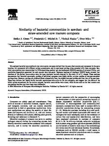
Adaptive Computational Chemotaxis in Bacterial Foraging Optimization: An Analysis Sambarta Dasgupta , Swagatam Das, Ajith Abraham, and Arijit Biswas
Abstract In his seminal paper published in 2002, Passino pointed out how individual and groups of bacteria forage for nutrients and how to model it as a distributed optimization process, which he called the Bacterial Foraging Optimization Algorithm (BFOA). One of the major driving forces of BFOA is the chemotactic movement of a virtual bacterium, which models a trial solution of the optimization problem. This article presents with a mathematical analysis of the chemotactic step in BFOA from the viewpoint of the classical gradient descent search. The analysis points out that the chemotaxis employed by classical BFOA, may result in sustained oscillation, especially on flat fitness landscapes, when a bacterium cell is near to the optima. To accelerate the convergence speed of the group of bacteria near global optima, two simple schemes for adapting the chemotactic step-height have also been proposed. Computer simulations over several numerical benchmarks indicate that BFOA with the adaptive chemotactic operators shows better convergence behavior as compared to the classical BFOA. Keywords: Biological systems, bacterial foraging, gradient descent search, computational chemotaxis, global optimization.
1 Introduction To tackle complex search problems of real world, scientists have been looking into the nature for years, both as model and as metaphor, for inspiration. Optimization is at the heart of many natural processes like Darwinian evolution, group behavior of social insects and the foraging strategy of other microbial creatures. Natural selection tends to eliminate species with poor foraging strategies and favor the propagation of genes of species with successful foraging behavior since they are more likely to enjoy reproductive success. Since a foraging organism or animal takes necessary action to maximize the energy utilized per unit time spent for foraging, considering all the constraints presented by its own physiology such as sensing and cognitive capabilities, environment (e.g. density of prey, risks from predators, physical characteristics of the search space), the natural foraging strategy can lead to optimization and essentially this idea can be applied to solve real-world optimization problems. Based on this conception, Passino proposed an optimization technique known as the Bacterial Foraging Optimization Algorithm (BFOA) [1, 2]. Until date, BFOA has successfully been applied to real world problems like optimal controller design [1, 3], harmonic estimation [4], transmission loss reduction [5], active power filter synthesis [6], and machine learning [7]. One major step in BFOA is the simulated chemotactic movement. Chemotaxis is a foraging strategy that implements a type of local optimization where the bacteria try to climb up the nutrient concentration to avoid noxious substance and search for ways out of neutral media. This step has much resemblance with a biased random walk model [8].
This article provides a mathematical analysis of the simulated chemotaxis in the light of the classical gradient descent search [9, 10] algorithm. The analysis reveals that a chemotactic step-height varying as the function of the current fitness value, can lead to better convergence behavior as compared to a fixed step-height. The adaptation schemes, proposed for automatically adjusting the step-height, are simple and impose no additional computational burden on the BFOA in terms of excess number of Function Evaluations (FEs). The proposed Adaptive BFOA (ABFOA) schemes have been compared with their classical counterpart, a very popular swarm-intelligence algorithm known as the Particle Swarm Optimization (PSO) [11] and a standard real-coded Genetic Algorithm (GA) [12, 13] over a test bed of ten numerical benchmarks with respect to the following performance measures: solution quality, convergence speed and the frequency of hitting the optimal solution. The paper finally investigates an interesting application of the ABFOA schemes to a realworld optimization problem arising in the field of communication engineering. The rest of the paper is organized as follows. In section 2, we outline the classical BFOA in sufficient details. Section 3 reviews the existing research-works on BFOA. Section 4 provides a mathematical analysis of the chemotactic movement of a simple, one-dimensional bacterium and proposes the adaptive chemotactic operators for BFOA. Section 5 provides detailed comparison between the classical BFOA and ABFOA over a test-suit of well-known numerical benchmarks. Section 6 describes an application of the adaptive BFOA variants to the parameter estimation for frequency-modulated sound wave. Finally conclusions are drawn in section 7. Analysis of the chemotaxis for a multi-bacterial system has been presented in Appendix I. It has also been shown that under certain conditions the mathematical model of the multi-bacterial system boils down to that of a single bacterium.
2. The Classical BFOA algorithm The bacterial foraging system consists of four principal mechanisms, namely chemotaxis, swarming, reproduction and elimination-dispersal [1]. Below we briefly describe each of these processes and finally provide a pseudo-code of the complete algorithm. i)
Chemotaxis: This process simulates the movement of an E.coli cell through swimming and tumbling via flagella. Biologically an E.coli bacterium can move in two different ways. It can swim for a period of time in the same direction or it may tumble, and alternate between these two modes of operation for the entire lifetime. Suppose θ i ( j , k , l ) represents i-th bacterium at j-th chemotactic, k-th reproductive and l-th elimination-dispersal step. C(i) is the size of the step taken in the random direction specified by the tumble (run length unit). Then in computational chemotaxis the movement of the bacterium may be represented by ∆ (i ) (1) θ i ( j + 1, k , l ) = θ i ( j , k , l ) + C (i ) T ∆ (i )∆ (i ) Where ∆ indicates a vector in the random direction whose elements lie in [-1, 1].
ii)
Swarming: An interesting group behavior has been observed for several motile species of bacteria including E.coli and S. typhimurium, where stable spatio-temporal patterns (swarms) are formed in semisolid nutrient medium. A group of E.coli cells arrange themselves in a traveling ring by moving up the nutrient gradient when placed amidst a semisolid matrix with a single nutrient chemo-effecter. The cells when stimulated by a high level of succinate, release an attractant aspertate, which helps them to aggregate into groups and thus move as concentric patterns of swarms with high bacterial density. The cell-to-cell signaling in E. coli swarm may be represented by the following function.
S
J cc (θ , P( j, k , l )) = ∑ J cc (θ ,θ i ( j, k , l )) i =1 S
p
S
p
i =1
m=1
i =1
m=1
= ∑[−d attractant exp(−wattractant∑ (θ m − θ mi ) 2 )] +∑[hrepellant exp(−wrepellant∑ (θ m − θ mi ) 2 )] (2) where J cc (θ , P ( j , k , l )) is the objective function value to be added to the actual objective function (to be minimized) to present a time varying objective function, S is the total number of bacteria, p is the number of variables to be optimized, which are present in each bacterium and θ = [θ 1,θ 2,...................,θ p ]T is a point in the p-dimensional search domain.
d aatractant , wattractant , hrepellant , wrepellant are different coefficients that should be chosen properly. iii) Reproduction: The least healthy bacteria eventually die while each of the healthier bacteria (those yielding lower value of the objective function) asexually split into two bacteria, which are then placed in the same location. This keeps the swarm size constant. iv) Elimination and Dispersal: Gradual or sudden changes in the local environment where a bacterium population lives may occur due to various reasons e.g. a significant local rise of temperature may kill a group of bacteria that are currently in a region with a high concentration of nutrient gradients. Events can take place in such a fashion that all the bacteria in a region are killed or a group is dispersed into a new location. To simulate this phenomenon in BFOA some bacteria are liquidated at random with a very small probability while the new replacements are randomly initialized over the search space. The pseudo-code as well as the flow chart (Figure 1) of the complete algorithm is detailed below: The BFOA Algorithm Parameters: i
[Step 1] Initialize parameters p, S, Nc, Ns, Nre, Ned, Ped, C(i)(i=1,2…S), θ . Where, p: Dimension of the search space, S: Total number of bacteria in the population, Nc : The number of chemotactic steps, Ns: The swimming length. Nre : The number of reproduction steps, Ned : The number of elimination-dispersal events, Ped : Elimination-dispersal probability, C (i): The size of the step taken in the random direction specified by the tumble. Algorithm: [Step 2] Elimination-dispersal loop: l=l+1 [Step 3] Reproduction loop: k=k+1 [Step 4] Chemotaxis loop: j=j+1 [a] For i =1,2…S take a chemotactic step for bacterium i as follows. [b] Compute fitness function, J (i, j, k, l). Let, J (i,
j , k , l ) = J (i, j , k , l ) + J cc (θ i ( j , k , l ), P ( j , k , l )) (i.e. add on the cell-to cell
attractant–repellant profile to simulate the swarming behavior)
where, Jcc is defined in (2). [c] Let Jlast=J (i, j, k, l) to save this value since we may find a better cost via a run. p
[d] Tumble: generate a random vector ∆ (i ) ∈ ℜ with each element
∆ m (i ), m = 1,2,..., p, a
random number on [-1, 1]. [e] Move: Let
∆ (i )
θ i ( j + 1, k , l ) = θ i ( j , k , l ) + C (i )
T
∆ (i ) ∆ (i ) This results in a step of size C (i ) in the direction of the tumble for bacterium i. [f] Compute J (i, j + 1, k , l ) and let
J (i, j + 1, k , l ) = J (i, j , k , l ) + J cc (θ i ( j + 1, k , l ), P ( j + 1, k , l )) . [g] Swim i) Let m=0 (counter for swim length). ii) While m< N s (if have not climbed down too long). • Let m=m+1. • If J (i, j + 1, k , l ) < Jlast ( if doing better), let Jlast = J (i, j + 1, k , l ) and let
θ i ( j + 1, k , l ) = θ i ( j , k , l ) + C (i ) And use this
θ i ( j + 1, j , k )
∆ (i ) ∆T (i ) ∆ (i )
to compute the new J (i, j + 1, k , l ) as we did in [f]
• Else, let m= N s . This is the end of the while statement. [h] Go to next bacterium (i+1) if i ≠ S (i.e., go to [b] to process the next bacterium). [Step 5] If j < N c , go to step 4. In this case continue chemotaxis since the life of the bacteria is not over. [Step 6] Reproduction: [a] For the given k and l, and for each i = 1,2,..., S , let N c +1 i J health =
∑ J (i, j, k , l )
(3)
j =1
be the health of the bacterium i (a measure of how many nutrients it got over its lifetime and how successful it was at avoiding noxious substances). Sort bacteria and chemotactic parameters C (i ) in order of ascending cost J health (higher cost means lower health). [b] The S r bacteria with the highest J health values die and the remaining S r bacteria with the best values split (this process is performed by the copies that are made are placed at the same location as their parent). [Step 7] If k < N re , go to step 3. In this case, we have not reached the number of specified reproduction steps, so we start the next generation of the chemotactic loop. [Step 8] Elimination-dispersal: For i = 1,2..., S with probability Ped , eliminate and disperse each bacterium (this keeps the number of bacteria in the population constant). To do this, if a bacterium is eliminated, simply disperse another one to a random location on the optimization domain. If l < N ed , then go to step 2; otherwise end.
Fig. 1: Flowchart of the Bacterial Foraging Algorithm
3. Related Works on BFOA Since its advent in 2002, BFOA has attracted the researchers from diverse domains of knowledge. This resulted into a few variants of the classical algorithm as well as many interesting applications of the same to the real-world optimization problems. In 2002, Liu and Passino [2] incorporated a new function J ar (θ ) in BFOA to represent the environment-dependent cell-to-cell signaling, such that
J ar (θ ) = exp( M − J (θ )).J cc (θ ) where M is a tunable parameter and minimization of J (i,
(4)
J cc (θ ) is given by (2). For swarming, they considered the
j , k , l ) + J ar (θ i ) .
In [14], Tang et al. model the bacterial foraging behaviors in varying environments. Their study focused on the use of individual-based modeling (IbM) method to simulate the activities of bacteria and the evolution of bacterial colonies. They derived a bacterial chemotaxis algorithm in the same framework and showed that the proposed algorithm can reflect the bacterial behaviors and population evolution in varying environments, through simulation studies. Li et al. proposed a modified Bacterial Foraging Algorithm with Varying Population (BFAVP) [15] and applied the same to the Optimal Power Flow (OPF) problems. Instead of simply describing chemotactic behavior into BFOA as done by Passino [1], BFAVP also incorporates the mechanisms of bacterial proliferation and quorum sensing, which allow a varying population in each generation of bacterial foraging process. Tripathy and Mishra proposed an improved BFO algorithm for simultaneous optimization of the real power losses and Voltage Stability Limit (VSL) of a mesh power network [16]. In their modified algorithm, firstly, instead of the average value, the minimum value of all the chemotactic cost functions is retained for deciding the bacterium’s health. This speeds up the convergence, because in
the average scheme described by Passino [1], it may not retain the fittest bacterium for the subsequent generation. Secondly for swarming, the distances of all the bacteria in a new chemotactic stage are evaluated from the globally optimal bacterium to these points and not the distances of each bacterium from the rest of the others, as suggested by Passino [1]. Simulation results indicated the superiority of the proposed approach over classical BFOA for the multi-objective optimization problem involving the UPFC (Unified Power Flow Controller) location, its series injected voltage, and the transformer tap positions as the variables. Mishra and Bhende used the modified BFOA to optimize the coefficients of Proportional plus Integral (PI) controllers for active power filters. The proposed algorithm was found to outperform a conventional GA [6] with respect to the convergence speed. Mishra, in [4], proposed a Takagi-Sugeno type fuzzy inference scheme for selecting the optimal chemotactic step-size in BFOA. The resulting algorithm, referred to as Fuzzy Bacterial Foraging (FBF), was shown to outperform both classical BFOA and a Genetic Algorithm (GA) when applied to the harmonic estimation problem. However, the performance of the FBF crucially depends on the choice of the membership function and the fuzzy rule parameters [4] and there is no systematic method (other than trial and error) to determine these parameters for a given problem. Hence FBF, as presented in [4], may not be suitable for optimizing any benchmark function in general. Hybridization of BFOA with other naturally inspired meta-heuristics has remained an interesting problem for the researchers. In this context, Kim et al. proposed a hybrid approach involving GA and BFOA for function optimization [3]. The proposed algorithm outperformed both GA and BFOA over a few numerical benchmarks and a practical PID controller design problem. Biswas et al. proposed a synergism of BFOA with another very popular swarm intelligence algorithm well known as the Particle Swarm Optimization (PSO) [17]. The new algorithm, named by the authors as Bacterial Swarm Optimization (BSO), was shown to perform in a statistically significantly better way as compared to both of its classical counterparts over several numerical benchmarks. Ulagammai et al. applied BFOA to train a Wavelet-based Neural Network (WNN) and used the same for identifying the inherent non-linear characteristics of power system loads [18]. In [19], BFOA was used for the dynamical resource allocation in a multiple input/output experimentation platform, which mimics a temperature grid plant and is composed of multiple sensors and actuators organized in zones. Acharya et al. proposed a BFOA based Independent Component Analysis (ICA) [20] that aims at finding a linear representation of non-gaussian data so that the components are statistically independent or as independent as possible. The proposed scheme yielded better mean square error performance as compared to a CGAICA (Constrained Genetic Algorithm based ICA). Chatterjee et al. reported an interesting application of BFOA in [21] to improve the quality of solutions for the extended Kalman Filters (EKFs), such that the EKFs can offer to solve simultaneous localization and mapping (SLAM) problems for mobile robots and autonomous vehicles. To the best of our knowledge, none of the existing works has, however, attempted to develop a fullfledged mathematical model of the bacterial foraging strategies for investigating important issues related to convergence, stability and oscillations of the foraging dynamics near global optima. The present work may be considered as a first, humble contribution in this context.
4. A Simple Algebraic Analysis of the Computational Chemotaxis Let us consider a single bacterium cell that undergoes chemotactic steps according to (1) over a onedimensional objective function. The bacterium lives in continuous time and at the t-th instant its position is given by, which is a real number. Let the objective function to be minimized 2
be J ( x ) = x . Below we list a few assumptions that were considered for the sake of gaining mathematical insight into the process. i) The objective function J (x ) is continuous and differentiable at all points in the search space.
ii) The chemotactic step size C is not very large (Passino himself took C = 0.1 ) iii) The analysis applies to the regions of the fitness landscape where gradients of the function are small i.e. near to the optima. According to assumption (iii), the analysis will be restricted within regions like the shaded one in Figure 2. In Figure 2, the dashed-line arrow represents velocity of the bacterium and the blue arrow shows the gradient vector. We note that the velocity vector does not necessarily coincide with the gradient vector. Initially, the bacterium was at point P and it moves to point Q. Here, the vector PQ shows the direction of velocity of the bacterium.
Fig. 2: A continuous, one-dimensional fitness landscape for BFOA. The analysis presented here holds perfect for regions like the shaded one.
4.1 Analytical Treatment Let the position of an individual bacterium at time t be θ (t ) and value of objective function J (θ ) . As
θ (t ) is a function of time then J (θ ) is a function of time. The bacterium may change its position continuously with time, which in turn may change its objective function value. Computer simulation of the algorithm, however, proceeds through discrete iterations (chemotactic steps). Certain amount of processor time is elapsed between two successive iterations. Thus, in the virtual world of simulations, a bacterium can change its position only at certain discrete time instants. This change of position is ideally instantaneous. In between two successive iterations the bacterium remains practically immobile. Without losing generality, the time between two successive iterations may be defined as unit time for the following derivation. The situation is depicted in Figure 3, where the bacterium changes its position instantly at certain discrete time points. But we have assumed that the bacterium lives in continuous time, where it is not possible to have instantaneous position change. Hence, we assume within two successive iterations the position shifts continuously and linearly (e.g. for time intervals (2-3), (4-5), (8-9)). In practice, time between two successive iterations i.e. computational time of iteration is very small. This ensures that the linear approximation is fairly good.
Fig. 3: Bacterium changing positions instantaneously and its approximated counterpart
Let us assume that, after an infinitesimal time interval ∆t , its position changes by an amount ∆θ from θ (t ) when the objective function value becomes smaller for changed position. Figure 4 reveals the nature of the time rate of change of position of the bacterium. We can now define the velocity of the bacterium as,
Vb = Lim ∆t → 0
∆θ ∆t
Naturally, here we assume the time to be unidirectional (i.e. ∆t
(5)
> 0)
Fig. 4: variation of velocity with successive iterations
From Figure 4 it can be observered that the velocity of bacterium is a train of pulses occuring at certain points of time. As the pulse width is diminished its height is increased. Ideally position changes instanteneously making height of the pulse tending towards infinity. Irregardless of the pulse width, area under the rectangle is always equals to step height C (0.1 in this case). As we assume velocity to be constant over the complete interval (i.e. position changes uniformly), its magnitude becomes C . In Figure 3 and Figure 4, iterations signify successive chemotactic steps taken by the bacterium. Time between two consecutive iterations is elapsed in necessary computation associated with one step. Now, according to BFOA, the bacterium changes its position only if the modified objective function value is less than the previous one i.e. J (θ ) > J (θ + ∆θ ) i.e. J (θ ) - J (θ + ∆θ ) is positive. This ensures that bacterium always moves in the direction of decreasing objective function value. In this analysis we denote the unit vector along the direction of tumble by ∆ , i.e. ∆ here is analogous to the unit vector ∆ (i )
∆T (i).∆(i )
in equation (1) as used by Passino for a multi-dimensional
fitness landscape. Please note that for a one-dimensional problem, ∆ is of unit magnitude and hence can assume only two values 1 or –1 with equal probabilities. Thus its value would remain unchanged after dividing it by square of its amplitude (as done in step 4[e] of the classical BFO algorithm). The bacterium moves by an amount of C∆ if objective function value is reduced for new location. Otherwise, its position will not change at all. Assuming uniform rate of position change, if the bacterium moves C∆ in unit time, its position is changed by (C∆ )(∆t ) in ∆t sec. It decides to move in the direction in which concentration of nutrient increases or in other words objective function decreases i.e. J (θ ) − J (θ + ∆θ ) > 0 . Otherwise it remains immobile. We have assumed that ∆t is an infinitesimally small positive quantity, thus sign of the quantity J (θ ) − J (θ + ∆θ ) remains unchanged if ∆t divides it. So, bacterium will change its position if and only if
J (θ ) − J (θ + ∆θ ) is positive. This crucial decision making (i.e. whether to take a step or not) ∆t activity of the bacterium can be modeled by a unit step function (also known as Heaviside step function [23]) defined as, u ( x ) = 1 , if x > 0; (6) = 0, otherwise.
J (θ ) − J (θ + ∆θ ) ).(C.∆ )( ∆t ) , where value of ∆θ is 0 or (C∆ )(∆t ) ∆t according to value of the unit step function. Dividing both sides of above relation by ∆t we get, ∆θ J (θ ) − J (θ + ∆θ ) = u[ ]C.∆ ∆t ∆t ∆θ {J (θ + ∆θ ) − J (θ )} ⇒ = u[− ]C.∆ (7) ∆t ∆t
Thus, ∆θ = u (
From (5) we have,
J (θ + ∆θ ) − J (θ ) ∆θ = Lim[u{− }.C.∆] ∆ t → 0 ∆t ∆t J (θ + ∆θ ) − J (θ ) ∆θ ⇒ Vb = Lim[u{− }.C.∆ ] ∆t → 0 ∆θ ∆t Vb = Lim ∆t → 0
as ∆t → 0 makes ∆θ
→ 0 , we may write, J (θ + ∆θ ) − J (θ ) ∆θ Vb = [u{− Lim Lim }.C.∆ ] ∆θ → 0 ∆θ ∆t →0 ∆t J (θ + ∆θ ) − J (θ ) Again, J (x ) is assumed to be continuous and differentiable. Lim is the ∆θ →0 ∆θ dJ (θ ) value of the gradient at that point and may be denoted by or G . Therefore we have: dθ Vb = u (−GVb )C∆
(8)
dJ (θ ) = gradient of the objective function at θ. In (8) argument of the unit step dθ function is −GVb . Value of the unit step function is 1 if G and Vb are of different sign and in this case the velocity is C∆ . Otherwise, it is 0 making bacterium motionless. So (8) suggests that bacterium will move the direction of negative gradient. Since the unit step function u ( x ) has a jump discontinuity at x = 0 , to simplify the analysis further, we replace u ( x ) with the continuous logistic function φ ( x ) , where 1 φ ( x) = 1 + e − kx 1 We note that, u ( x) = Lt φ (x) = Lt (9) k →∞ k →∞ 1 + e − kx
where,
G=
Figure 5 illustrates how the logistic function may be used to approximate the unit step function used for decision-making in chemotaxis. For analysis purpose k cannot be infinity. We restrict ourselves to moderately large values of k (say k = 10) for which φ (x ) fairly approximates u (x ) . Subsection 4.3 describes the error limit introduced by this assumption. Thus, for moderately high values of k φ (x) fairly approximates u (x). Hence from (8),
Vb =
C∆ 1 + e kGVb
(10)
Fig. 5: The unit step and the logistic functions
According to assumptions (ii) and (iii), if C and G are very small and k ~10, then also we may have | kGVb | <<1.In that case we neglect higher order terms in the expansion of
e kgvb and
have
e kgvb ≈ 1 + kGVb . Substituting it in (10) we obtain, Vb =
C .∆ 2 + kGV
C .∆ = 2
⇒ Vb
⇒ Vb =
b
1 kGV 1+ 2
kGV b C .∆ (1 − ) 2 2
b
[Θ |
kGVb |<<1, neglecting higher 2
terms, (1 +
kGV b −1 kGV b ) ≈ (1 − )] 2 2
After some manipulation we have,
2 C .∆ 4 + kGC . ∆ C∆ 1 ⇒ Vb = kCG ∆ 2 1+ 4 C∆ kGC ∆ ⇒ Vb = (1 − ) 2 4
(11)
Vb =
[Θ |
kGC∆ kGC |=| | <<1, as ∆ = 1 and 4 4
neglecting the higher order terms.] 2
⇒ Vb =
2
C∆ kGC ∆ − 2 8
⇒ Vb = −
kC 8
2
G +
C∆ 2
[Θ
∆2 = 1 ]
(12)
Equation (12) is applicable to a single bacterium system and it does not take into account the cell-tocell signaling effect. A more complex analysis for the two-bacterium system involving the swarming effect has been included at the appendix. It indicates that, a complex perturbation term is added to the dynamics of each bacterium due to the effect of the neighboring bacteria cells. However, the term becomes negligibly small for small enough values of C (~0.1) and the dynamics under these circumstances get practically reduced to that described in (12). In what follows, we shall continue the analysis for single bacterium system for better understanding of the chemotactic dynamics.
4.2 Experimental Verification of Characteristic Equation of Chemotaxis Characteristic equation of chemotaxis (12) represents the dynamics of bacterium taking chemotactic steps. In order to verify how reliably the equation represents the motion of the virtual bacterium compare results obtained from (12) with that of according to BFOA. First the equation is expressed in iterative form, which is, kC 2 C ∆ (n ) V b ( n ) = θ ( n ) − θ ( n − 1) = − G ( n − 1) + 8 2
⇒ θ ( n ) = θ ( n − 1) −
kC 8
2
G ( n − 1) +
C ∆ (n ) 2
(13)
where n is the iteration index. The tumble vector is also a function of iteration count (i.e. chemotactic step number) i.e. it is generated repeatedly for successive iterations. We have taken
J (θ ) = θ 2 as objective function for this experimentation. Bacterium was initialized at –2 i.e. θ (0) = −2 and C is taken as 0.2. Gradient of J (θ ) is 2θ . Therefore G (n − 1) may be replaced by 2θ ( n − 1) .Finally for this specific case we get, θ ( n ) = (1 −
kC 2 C ∆ (n) )θ ( n − 1) + 4 2
(14)
We compute values of θ (n) for successive iterations according to above iterative relation. Also values of positions are noted following guidelines of BFOA. With current position is changed by C∆ if objective function value decreases for new position. Results have been presented in Figure 6. Figure 6 (a) shows position in successive iteration according to BFOA and as obtained from (14). Here also we have assumed position of bacterium changes linearly between two consecutive iterations. Mismatch between actual and predicted values is also shown. In Figure 6(b) actual and predicted values of velocity is shown. Velocity is assumed to be constant between two successive iterations. According to BFOA magnitude of velocity is either C (0.2 in this case) or 0. Difference between actual and predicted velocity is shown as error. Time lapsed between two consequent iterations is spent for computation and is termed as unit time. This may be perceived as the time required by a bacterium to measure nutrient content of a new point on fitness landscape. Actually it is the time taken by the processor to perform numerical computations.
(a) Graphs showing actual, predicted positions of bacterium and error in estimation over successive iterations.
(b) Similar plots for velocity of the bacterium. Fig. 6: Comparison between actual and predicted motional state of the bacterium.
4.3 Estimation of Error and Limitations of the Analysis. Due to the approximation of the unit step function, small error has been introduced in the analysis. Again we have simplified the function for some special cases (assumption (ii) and (iii)). Here, magnitude of maximum possible value of error in estimation of Vb equals | C∆ |= C .Θ| ∆ |= 1 . 2
According to (9) we may replace
u (x) approximately by the logistic function ϕ ( x) =
2
1 , for 1 + e − kx
moderately high value of k. If x is small, we may again approximate the logistic function with the following equation of a straight line as:
ϕ (x) =
1 k x+ 4 2
(15)
φ(x)
Fig. 7: The region of error due to approximation of the unit step with the logistic functions
These simplifications have already been undertaken in expressions (10) to (12) of section 4.1, where x = GVb . The straight line, which approximates the logistic function as shown in Figure 7,
intersects graph of the logistic function at two points A and B. When |x| > OA or |x| > OC, the error in decision-making term of our analysis gradually increases. So we must restrict the analysis within the region AC i.e. magnitude of GVb has certain limits. As shown in Figure 7, x must lie between A and C i.e. ϕ (x) should be restricted within the range [0, 1], or otherwise considerable error creeps into the analysis. After imposing these constraints on (15) we get, k 1 k 1 (16) x + ≤ 1 and x + ≥ 0 4 2 4 2 After solving above couple of inequalities we finally obtain
2 . k
(17)
2 k |G|
(18)
2 C∆ kC 2 ≥| Vb |=| − G| k |G| 2 8
(19)
x≤ Substituting, x by
GVb in (17), | Vb |≤
From (12) and the above inequality we get,
We know for any two numbers
a and b , | a − b |≥| a |~| b | . Hence, 2
2
|
C kC C∆ kC C∆ kC 2 | G |. − G |≥ | |−| G |= − 2 8 2 8 2 8
[C
> 0, k > 0 and ∆ can
assume
values 1 and –1 randomly, giving | ∆ |= 1 ] Incorporating inequality (19) in the above,
2 C∆ kC 2 C kC 2 ≥| − G| ≥ − |G| 2 8 k |G| 2 8 Again, as,
|
(20)
| a − b |≥| b | − | a |
kc 2 C∆ kC 2 C C∆ kC 2 G|−| |= |G|− − G |≥ | 2 8 8 2 8 2
Incorporating inequality (19) in above we further get,
kC C∆ kC 2 2 − G |≥ ≥| 2 8 8 k |G|
2
|G|−
C 2
(21)
Inequality (20) implies, 2 2 ≥ C − kC | G | 8 k |G | 2
⇒ (k | G | C − 2) 2 + 12 ≥ 0 , which is trivially true. From inequality (21) we get,
C 2 kC 2 ≥ |G| − k |G | 2 8 ⇒ k 2 | G | 2 C 2 − 4k | G | C − 16 ≤ 0 2 2 ⇒− ( 5 − 1) ≤ C ≤ (1 + 5 ) k |G| k |G| But since C
> 0, 0
2 (1 + 5 ) k |G|
(22)
Now, let us assume within our domain of analysis
| G | max be the maximum possible magnitude of
2 (1 + 5 ) term is minimized when | G |=| G | max . Our analysis is valid if k |G | 2 chemotactic step size is less than or equals to this minimum value i.e. (1 + 5 ) . So we k | G | max 2 define maximum allowable value of chemotactic step size as C max = (1 + 5 ) . If k | G | max
gradient.
| G | max is large maximum allowable step size almost vanishes making our analysis invalid for moderately small values of step size. From this consideration also we should restrict domain of analysis within the region with moderate value of gradient. 4.4 Chemotaxis and the Classical Gradient Decent Search From expression (12) of section 4.1, we get
kC 2 C∆ dθ (23) G+ ⇒ = −α / G + β / 8 2 dt 2 C∆ / / . The classical gradient descent search algorithm is given by the where α is − kC and β is 2 8 Vb = −
following dynamics in single dimension [10]:
dθ = −α .G + β dt where,
α
is the learning rate and
β
(24) is the momentum. Similarity between (23) and (24) suggests /
that chemotaxis may be considered a modified gradient descent search, where α , a function of chemotactic step-size can be identified as the learning rate parameter.
Fig. 8: A sample fitness landscape for studying the computational chemotaxis
Already we have discussed in section 4.3 that magnitude of gradient should be small within the region of our analysis. So we choose point P in the one dimensional fitness landscape shown in Figure 8 as the operating point for our analysis. For chemotaxis of BFOA, when G becomes very small, the gradient descent term term
α / G of equation (23) becomes ineffective. But the random search
C∆ plays an important role in this context. From equation (23), considering G → 0 , we have 2
dθ C ∆ = ≠0 dt 2
(25)
So there is a convergence towards actual minima. Figure 8 shows a region on fitness landscape with very small value of gradient. The random search or momentum term C∆ in the RHS of equation 2 (12) provides an additional feature to the classical gradient descent search. When gradient becomes very small, the random term dominates over gradient decent term and the bacterium changes its position. But random search term may lead to change in position in the direction of increasing objective function value. If it happens then again magnitude of gradient increases and dominates the random search term. 4.5 Oscillation Problem: Need for Adaptive Chemotaxis If magnitude of the gradient decreases consistently, near the optima or very close to the optima
α /G
of expression (23) becomes comparable to β . Then gradually β becomes dominant. When | G |→ 0, | dθ |≈| β |=| C∆ |= C Θ | ∆ |= 1 . Let us assume the bacterium has reached close to dt 2 2 the optimum. But since we obtain | dθ |= C , the bacterium does not stop taking chemotactic steps dt 2 and oscillates about the optima. This crisis can be remedied if step size C is made adaptive according to the following relation,
C=
| J (θ ) | 1 = | J (θ ) | +λ 1 + λ J (θ )
(26)
where λ is a positive constant. Choice of a suitable value for λ has been discussed in the next subsection. Here we have assumed that the global optimum of the cost function is 0. Thus from (25) we see, if J (θ ) → 0 , then C → 0 . So there would be no oscillation if the bacterium reaches optima because random search term vanishes as C → 0 . The functional form given in equation (25) causes C to vanish nears the optima. Besides, it plays another important role described below. From (25), we have, when
J (θ ) is large
λ → 0 and consequently C → 1 . | J (θ ) |
The adaptation scheme presented in equation (26) has an important physical significance. If magnitude of cost function is large for an individual bacterium, it is in the vicinity of noxious substance. It will then try to move to a place with better nutrient concentration by taking large steps. On the other hand the bacterium, when in nutrient rich zone i.e. with small magnitude of the objective function value, tries to retain its position. Naturally, its step size becomes small. 4.6 Adaptive Chemotaxis for Avoiding the Lock-in State Let us consider an even function J (θ ) (as shown in Figure 9), which has its minima at θ = 0 and its minimum value is also equals to 0. Let us also assume the function is increasing in the interval
J (θ ) = θ 2 is an even function where it is increasing in the interval (0, ∞ ), and decreasing in (−∞,0) so in this case ϕ → ∞ ). A special case of stagnation may occur within the region ( − ϕ , ϕ ) . We here refer to this situation as lock in. The lock in
[0, ϕ ] and decreasing in [ − ϕ ,0 ] (e. g.
condition arises when a bacterium has reached somewhat near to the optima of a function and then its further movements are not possible due to comparatively large step size.
Example 1:
Suppose we have to minimize a one-dimensional function J (θ ) been provided in Figure 9.
Fig. 9: Fitness landscape for the function
= θ 2 . A plot of the function has
J (θ ) = θ 2
Let, in Figure 9, |PO|=|QO|= θ . We also assume that he bacterium is currently at the position
θ =θ
i.e. it is at Q. Now in classical chemotaxis, three cases may arise as described below:
Case I: Let step-size C
= 2 θ . Then, for ∆ = −1 , the bacterium should move to P. But as in this
case its objective function value remains same, it does not come to P, but stays at Q 2
[as J (θ ) = J ( −θ ) = θ ]. As ∆ = 1 tries to shift the bacterium to the right (where the objective function value increases again) it again stays at Q. Hence the bacterium gets trapped at Q. Case II: Let C
> 2 θ . In that case, bacterium remains immobile for both values of ∆. Here step
size is constant and greater than 2 × θ . If the bacteria moves in any one of the two directions, value of the objective function increases. So, bacterium is trapped. Case III: Let C
< 2 θ . In this case, bacterium will move to some point in the left of origin. But, C
is fixed (say, 0.5). So, after certain iterations any one of Case II and I must arise. The situation of the bacterium in these three cases has been depicted in Figure10.
(a) Case I
(b) Case II
(c) Case III
Fig. 10: Situation of a bacterium cell near the global optimum in classical chemotaxis. Now consider the situation where the step-size has been adapted according to (26). Then we have C =
θ2 θ2 +λ
. The lock-in states never occur if for all possible values of θ ,
C < 2 |θ | | θ |2 ⇒ < 2 |θ | | θ | 2 +λ
⇒
|θ | − | θ |2 2 consider f (| θ |) = | θ | − | θ | 2 . 2
⇒
Let
us
2
θ < 2 | θ | (| θ | 2 +λ )
[Θ
| θ | 2 +λ > 0
]
λ>
Maximum
value
of
function
is
obtained
when
1 1 df (| θ |) we get, = 0 ⇒ θ = . Putting, | θ |= 4 4 d |θ | 1 ) = 1 θ 4 16 Hence, for all values of θ , if λ > f (| θ |) ⇒ λ > 1 16 , then no trapping or sustained oscillations of arg max f (| θ |) = f (
the bacterium cell will arise near the global optimum. In this case the bacterium cell will follow a trajectory as depicted in Figure11.
Fig. 11: Convergence towards the global optima for adaptive step size in chemotaxis.
Next we provide a brief comparison between BFOA and the proposed ABFOA over the one-
= θ 2 . Each algorithm uses only a single bacterium and in both 1 the cases, it is initialized at θ (0) = 6.0 . We have taken λ > to avoid lock in. Results of 5 16 dimensional objective function J (θ )
iterations are tabulated in Table 1and the convergence characteristics has been graphically presented in Figure 12. Iteration signifies the chemotactic step number in this case. We can observe due to its constant step-size, the BFOA-bacterium stops before reaching optima. For ABFOA, the bacterium
adapts step-size according to objective function value and gradually nears optima. We get a better quality of final solution in this case. Table 1.Variation of bacterium position θ with chemotactic steps for adaptive step size C Chemotactic step number
According to BFOA
According to ABFOA1
θ
θ
1 2 3 4
0.600000 0.170000 0.170000 0.170000
0.600000 -0.175862 0.053353 0.053353
5
0.170000
0.026712
Fig. 12: Variation of bacterial position θ with time near the global optima for classical and adaptive chemotaxis.
4.7 A Special Case If the optimum value of the objective function is not exactly zero, step-size adapted according to (26) may not vanish near optima. Step-size would shrink if the bacterium come closer to the optima, but it may not approach zero always. To get faster convergence for such functions it becomes necessary to modify the adaptation scheme. Use of gradient information in the adaptation scheme i.e. making step-size a function of the function-gradient (say C = C ( J (θ ), G ) ) may not be practical enough, because in real-life optimization problems, we often deal with discontinuous and nondifferentiable functions. In order to make BFOA a general black-box optimizer, our adaptive scheme should be a generalized one performing satisfactorily in these situations too. Therefore to accelerate the convergence under these circumstances, we propose an alternative adaptation strategy in the following way:
C=
J (θ ) − J best J (θ ) − J best + λ
(27)
J best is the objective function value for the globally best bacterium (one with lowest value of objective function).
J (θ ) − J best is the deviation in fitness value of an individual bacterium from
global best. Expression (27) can be rearranged to give,
1
C= 1+
λ J (θ ) − J best
.
(28)
If
a
bacterium
making C ≈ 1Θ
is
far
λ J (θ ) − J best
apart
from
the
global
best,
J (θ ) − J best would be large
→ 0 . On the other hand if another bacterium is very close to it, step
size of that bacterium will almost vanish, because J (θ ) − J best becomes small and denominator of (28) grows very large. The scenario is depicted in Figure 13. In what follows, we shall refer the BFOA with adaptive scheme of equation (26) as ABFOA1 and the BFOA with adaptation scheme described in (27) will be referred as ABFOA2.
Fig. 13: An objective function with optimum value much greater than zero and a group of seven bacteria are scattered over the fitness landscape. Their step height is also shown.
Figure 13 shows how the step-size becomes large as objective function value becomes large for an individual bacterium. The bacterium with better function value tries to take smaller step and to retain its present position. For best bacterium of the swarm J (θ ) − J best is 0 . Thus, from (27) its stepsize is
1 , which is quite small. The adaptation scheme bears a physical significance too. A
λ
bacterium located at relatively less nutrient region of fitness landscape will take large step sizes to attain better fitness. Whereas, another bacterium located at a location, best in regard to nutrient content, is unlikely to move much. In real-world optimization problems, optimum value of the objective function is very often found to be zero. In those cases adaptation scheme of (26) works satisfactorily. But for functions, which do not have a moderate optimum value, (27) should be used for better convergence. Note that neither of two proposed schemes contains derivative of objective function so they can be used for discontinuous and non-differentiable functions as well.
5. Experiments and Results over Benchmark Functions This section presents an extensive comparison among the performances of two Adaptive BFOA schemes (ABFOA1 and ABFOA2), the classical BFOA, the BSO (Bacterial Swarm Optimization) algorithm, a standard real-coded GA and one of the state-of-the-art variants of the PSO algorithm. 5.1 Numerical Benchmarks Our test-suite includes ten well-known benchmark functions [23] of varying complexity. In Table 2, p represents the number of dimensions and we used p=15, 30, 45 and 60 for functions f1 to f7 while
functions f8 to f10 are two-dimensional. The first function is uni-modal with only one global minimum. The others are multi-modal with a considerable number of local minima in the region of interest. Table 2 summarizes the initialization and search ranges used for all the functions. An asymmetrical initialization procedure has been used here following the work reported in [24]. 5.2 Algorithms used for the Comparative Study and their Parametric Setup 5.2.1 The BFOA and its Adaptive Variants The original BFO and the two adaptive BFOA schemes employ the same parametric setup, except with the difference that the chemotactic step sizes in ABFOA1 and ABFOA2 have been made adaptive according to equations (25) and (26) respectively. After performing a series of hand-tuning experiments, we found that keeping λ = 4000 provides considerably good result for both the adaptive schemes over all benchmark functions considered here. The chemotactic step-size C (i ) was kept at 0.1 in the classical BFOA. Rest of the parameter settings that were kept same for these algorithms, have been provided in Table 3. In order to make the comparison fair enough, all runs of the three BFOA variants start from the same initial population over all the problem instances. 5.2.2 The HPSO-TVAC Algorithm Particle Swarm Optimization (PSO) [11, 25] is a stochastic optimization technique that draws inspiration from the behavior of particles, the boids method of Reynolds and socio-cognition. In classical PSO, a population of particles is initialized with random positions
ρ ρ X i and velocities Vi ,
and a function f is evaluated, using the particle’s positional coordinates as input values. In a Ddimensional search space,
ρ ρ X i = [ xi1 , xi 2 ,..., xiD ]T and Vi = [vi1 , vi 2 ,..., viD ]T .
Positions and velocities are adjusted, and an objective function is evaluated with the new coordinates at each time-step. The fundamental velocity and position update equations for the d-th dimension of the i-th particle in the swarm may be given as: vid (t + 1) = ω.vid (t ) + C1 .ϕ1 .( Pid − xid (t )) + C 2 .ϕ 2 .( Pgd − xid (t )) (29a)
xid (t + 1) = xid (t ) + vid (t + 1) The variables
ϕ1 and ϕ 2
restricted to an upper limit
(29b)
are random positive numbers, drawn from a uniform distribution and
ϕ max
(usually = 2) that is a parameter of the system.
called acceleration coefficients, whereas
ω
is known as inertia weight.
personal best solution found so far by an individual particle while
C1 and C 2 are
Pid is d-th component of the
Pgd represents d-th element of the
globally best particle found so far in the entire community.
Table 2. Description of the Benchmark Functions used
Function Sphere function (f1)
Mathematical Representation
Theoretical Optima
(-100, 100)p
ρ f 1 ( 0) = 0
(-100, 100)p
ρ f 2 (1) = 0
(-10, 10)p
ρ f 3 (0) = 0
(-600, 600)p
ρ f 4 ( 0) = 0
ρ 1 D 2 f 5 ( X ) = − 20 exp − 0 .2 ∑ xi − D i =1 D 1 exp ∑ cos 2π x i + 20 + e D i =1
(-32, 32)p
ρ f 5 (0) = 0
p ρ 2 f 6 ( X ) = ∑ (xi + 0.5)
(-100, 100)p
∑x
2 i
i =1
Rosenbrock (f2) Rastrigin (f3)
Range of search
p
ρ f1 ( x ) =
ρ f2 (x) = ρ f3 (x ) =
p −1
∑ [100 ( x
2
i +1
2
2
− x i ) + ( x i − 1) ]
i =1 p
∑
[x
2 i
− 10 cos( 2 π x i ) + 10 ]
i =1
Griewank (f4)
ρ f4 (x ) =
Ackley (f5)
Step (f6)
1 4000
p
p
∑
x
2 i
−
i =1
∏
cos(
i =1
xi ) +1 i
−
i =1
Schwefel’s Problem 2.22 (f7) Shekel’s Foxholes (f8)
ρ f 7 (X ) =
∑
xi +∏ xi
i =1
i =1
25
ρ 1 f8 ( x) = [ + 500
1
∑ j =1
1 1 ≤ pi < 2 2
ρ f 7 ( 0) = 0
(-500, 500)p
p
p
ρ f 6 ( p ) = 0,
2
j+
∑ (x
(-65.536, 65.536)2
] −1 i
− a ij ) 6
f 8 (−32,−32) = 0.998
i =1
ρ 1 f 9 ( X ) = 4 x12 − 2.1x14 + x16 + x1 x 2 − 4 x 22 + 4 x 26 3
Six-Hump CamelBack Function (f9) GoldsteinPrice Function (f10)
(-5,5)
f 9 (0.08983,−0.7126) = f 9 (−0.08983,0.7126) = −1.0316285
ρ 2 f 10 ( x ) = {1 + ( x 0 + x1 + 1) 2 (19 − 14 x 0 + 3 x 0
(-2, 2)2
2
− 14 x1 − 6 x 0 x1 + 3 x1 )}{ 30 + ( 2 x 0 − 3 x1 ) 2 2
f 10 (0,−1) = 3
2
(18 − 32 x 0 + 12 x 0 + 48 x1 − 36 x 0 x1 + 27 x1 )} Table 3. Common Parameter Setup for BFOA and Adaptive BFOA (ABFOA)
S 100
Nc 100
Ns 12
Ned 4
Nre 16
ped 0.25
dattractant 0.1
wattractant
wrepellant
hrepellant
λ
0.2
10
0.1
400
Ratnaweera et al. [26] recently suggested a parameter automation strategy for PSO where the cognitive component is reduced and the social component is increased (by varying the acceleration coefficients C1 and C 2 in (28a)) linearly with time. They suggested another modification, named self-organizing Hierarchical Particle Swarm Optimizer, in conjunction with the previously mentioned Time Varying Acceleration Coefficients (HPSO-TVAC). In this method, the inertial velocity term is kept at zero and the modulus of the velocity vector is reinitialized to a random velocity, known as “re-initialization velocity”, whenever the particle gets stagnant ( vid = 0 ) in some region of the search space. This way, a series of particle swarm optimizers are generated automatically inside the main particle system according to the behavior of the particles in the search space, until some stopping criterion is met. Here we compare this state-of-the-art version of PSO with the adaptive BFOA schemes. The parametric setup for HPSO-TVAC follows the work reported
ϖ
in [26]. The re-initialization velocity is kept proportional to the maximum allowable velocity Vmax . We fixed the number of particles = 40 and the inertia weight ω
= 0.794 . C1 was linearly increased ϖ from 0.35 to 2.4 while C2 was allowed to decrease linearly from 2.4 to 0.35. Finally, Vmax was set ρ at X max . 5.2.3 The Real-coded GA In this study, we used a standard real-coded GA (also known as Evolutionary Algorithm or EA [27]) that was previously found to work well on real-world problems [28]. The EA works as follows: First, all individuals are randomly initialized and evaluated according to a given objective function. Afterwards, the following process will be executed as long as the termination condition is not fulfilled: Each individual is exposed to either mutation or recombination (or both) operators with probabilities p m and p c respectively. The mutation and recombination operators used are Cauchy mutation with an annealing scheme and arithmetic crossover, respectively. Finally, tournament selection (of size 2) [27] is applied between each pair of individuals to remove the least fit members of the population. The Cauchy mutation operator is similar to the well-known Gaussian mutation operator, but the Cauchy distribution has thick tails that enable it to generate considerable changes more frequently than the Gaussian distribution. The Cauchy distribution may be presented as: 1 (30) C ( x,α , β ) = 2 x − α βπ 1 + β where α ≥ 0 , β > 0 and − ∞ < x < ∞ . An annealing scheme is employed to decrease the value of β as a function of the elapsed number of generation t while used the following annealing function:
β =
α as fixed to 0. In this work,
1 1+ t
we
(31)
In arithmetic crossover the offspring is generated as a weighted mean of each gene of the two parents, i.e.
offspring i = r. parent1i + (1 − r ). parent 2 i
(32)
The weight r is determined by a random value between 0 and 1. Here we fixed the population size at 100, p m = 0.9 and p c = 0.7 , respectively for all the problem instances. 5.2.4 The Bacterial Swarm Optimization (BSO) Biswas et al [17] proposed a hybrid optimization technique, which synergistically couples BFOA with PSO. The algorithm, referred to as the Bacterial Swarm Optimization (BSO), performs local search through the chemotactic movement operation of BFOA whereas the global search over the entire search space is accomplished by a PSO operator. In this way it balances between exploration and exploitation, enjoying best of both the worlds. In BSO, after undergoing a chemo-tactic step, each bacterium also gets mutated by a PSO operator. In this phase, the bacterium is stochastically attracted towards the globally best position found so far in the entire population at current time and also towards its previous heading direction. The PSO operator uses only the globally best position found by the entire population to update the velocities of the bacteria and eliminates term involving the personal best position as the local search in different regions of the search space is already taken care of by the chemo-tactic operator of BFOA. Parametric setup for the algorithm was kept exactly same as described in [17]. For the PSO operator we choose ω=0.8, C2=1.494 while for the BFO operators the parameter-values were kept as described in Table 3.
5.3 Simulation Strategy
The comparative study presented in this article, focuses on the following performance metrics: (a) the quality of the final solution (b) the convergence speed (measured in terms of the number of fitness function evaluations (FEs)) and (c) the frequency of hitting the optima. Fifty independent runs of each of the algorithms were carried out and the average and the standard deviation of the best-of-run values were recorded. For a given function of a given dimension, fifty independent runs of each of the six algorithms were executed, and the average best-of-run value and the standard deviation were obtained. Different maximum numbers of FEs was used according to the complexity of the problem. For benchmarks f1 to f7, the stopping criterion was set as reaching an objective function value of 0.001. However for f8, f9 and f10, the stopping criteria are fixed at 0.998, -1.0316 and 3.00 respectively. In order to compare the speeds of different algorithms, we note down the number of function evaluations (FEs) an algorithm takes to converge to the optimum solution (within the given tolerance). A lower number of FEs corresponds to a faster algorithm. We also keep track of the number of runs of each algorithm that manage to converge within the pre-specified error-limit over each problem. We employed unpaired t-tests to compare the means of the results produced by the best best ABFOA scheme and the best of the rest over each problem. Unpaired t-test assumes that the data has been sampled from a normally distributed population. From the concepts of central limit theorem, one may note that as sample sizes increase, the sampling distribution of the mean approaches a normal distribution regardless of the shape of the original population. A sample size around 50 allows the normality assumptions conducive for doing the unpaired t-tests [29]. 5.4 Empirical Results Table 4 compares the algorithms on the quality of the best solutions obtained. The mean and the standard deviation (within parentheses) of the best-of-run solution for 50 independent runs of each of the ten algorithms are presented in Table 4. Please note that in this table if all the runs of a particular algorithm converge to or below the pre-specified objective function value (=0.001for f1 to f6; 0.998, -1.0316 and 3.00 for f8, f9 and f10, respectively) within the maximum number of FEs, then we report this threshold value as the mean of 50 runs. Missing values of standard deviation in thses cases indicate a zero standard deviation. Table 5 shows results of unpaired t-tests between the best algorithm and the second best in each case (standard error of difference of the two means, 95% confidence interval of this difference, the t value, and the two-tailed P value). For all cases in Table 3, sample size = 50 and no. of degrees of freedom = 98. This table covers only those cases for which a single algorithm achieves the best accuracy of final results. Table 6 shows, for all test functions and all algorithms, the number of runs (out of 50) that managed to find the optimum solution (within the given tolerance) and also the average number of FEs taken to reach the optima along with the standard deviation (in parentheses). Missing values of standard deviation in this table also indicate a zero standard deviation. The entries marked as zero in this table indicate that no runs of the corresponding algorithm could manage to converge within the given tolerance in those cases. In all the tables, entries marked in bold represent the comparatively best results. The convergence characteristics of 6 most difficult benchmarks have been provided in Figure 14 for the median run of each algorithm (when the runs were ordered according to their final accuracies). Each graph shows how the objective function value of the best individual in a population changes with increasing number of FEs. Some of the illustrations were omitted in order to save space.
Table 4. Average and the standard deviation (in parenthesis) of the best-of-run solution for 50 independent runs tested on ten benchmark functions Func
Dim
Maximum No. of FEs
15
5×10⁴
30
1×10⁵
45
5×10⁵
60
1×10⁶
15
5×10⁴
30
1×10⁵
45
5×10⁵
60
1×10⁶
15
5×10⁴
30
1×10⁵
45
5×10⁵
60
1×10⁶
15
5×10⁴
30
1×10⁵
45
5×10⁵
60
1×10⁶
15
5×10⁴
30
1×10⁵
45
5×10⁵
60
1×10⁶
15
5×10⁴
30
1×10⁵
45
5×10⁵
60
1×10⁶
15
5×10⁴
30
1×10⁵
45
5×10⁵
60
1×10⁶
f8
2
1×10⁵
f9
2
1×10⁵
f10
2
1×10⁵
f1
f2
f3
f4
f5
f6
f7
Mean Best Value (Standard Deviation) BFOA 0.0086 (0.0044) 0.084 (0.0025) 0.776 (0.1563) 1.728 (0.2125) 36.595 (28.1623) 58.216 (14.3254) 96.873 (26.136) 154.705 (40.1632) 10.4521 (5.6632) 17.5248 (9.8962) 32.9517 (10.0034) 41.4823 (17.6639) 0.2812 (0.0216) 0.3729 (0.0346) 0.6351 (0.0522) 0.8324 (0.0764) 0.9332 (0.0287) 2.3243 (1.8833) 3.4564 (3.4394) 4.3247 (1.5613) 0.0400 (0.00283) 2.0802 (0.00342) 14.7328 (3.2827) 19.8654 (4.8271) 2.8271 (0.3029) 4.6354 (2.7753) 9.4563 (10.2425) 16.4638 (12.40940 1.056433 (0.01217) -0.925837 (0.000827) 3.656285 (0.109365)
HPSOTVAC 0.001
0.001
0.001
0.001
0.001
0.065 (0.0534) 0.383 (0.05564) 1.364 (0.5136) 94.472 (75.8276) 706.263 (951.9533) 935.2601 (1102.352) 1264.287 (1323.5284) 9.467 (3.726) 34.837 (10.128) 46.332 (22.4518) 58.463 (66.4036) 0.0564 (0.025810 0.2175 (0.1953) 0.4748 (0.4561) 0.7462 (0.5521) 0.1217 (0.0125) 0.5684 (0.1927) 0.9782 (0.2029) 2.0293 (3.7361) 0.001
0.036 (0.001) 0.257 (0.0323) 0.6351 (0.0298) 14.756 (10.5552) 31.738 (3.6452) 67.473 (16.3526) 109.562 (34.7275) 0.4981 (0.0376) 3.797 (0.8241) 8.536 (2.7281) 12.0922 (4.5631) 0.05198 (0.00487) 0. 2684 (0.3616) 0.3732 (0.0971) 0.6961 (0.4737) 0.001482 (0.00817) 0.6059 (0.3372) 0.9298 (0.7631) 1.8353 (1.4635) 0.001
0.056 (0.0112) 0.354 (0.2239) 0.775 (0.4291) 0.673 (0.1454) 15.471 (2.655) 30.986 (4.3438) 76.647 (24.5281) 0.2632 (0.2348) 13.7731 (3.9453) 18.9461 (7.7075) 10.2266 (2.8942) 0.1741 (0.097) 0.2565 (0.1431) 0.5678 (0.236) 0.7113 (0.097) 0.1025 (0.00347) 0.5954 (0.1246) 1.0383 (0.2542) 1. 9166 (0.536) 0.001
0.022 (0.00625) 0.208 (0.0664) 0.427 (0.1472) 11.561 (2.355) 4.572 (3.0631) 24.663 (10.8644) 91.257 (32.6283) 0.3044 (0.6784) 2.5372 (0.3820) 6.0236 (1.4536) 8.3343 (0.2917) 0.0321 (0.02264) 0.1914 (0.0117) 0.3069 (0.0526) 0.5638 (0.3452) 0.7613 (0.0542) 0.5038 (0.5512) 1.5532 (0.1945) 1.7832 (0.4581) 0.001
0.044 (0.0721) 0.419 (0.2096) 0.632 (0.5747) 15.4931 (4.3647) 6.748 (2.6625) 39.736 (30.6261) 84.6473 (53.2726) 2.6573 (0.0372) 2.9823 (0.5719) 8.1121 (4.3625) 9.4637 (6.7921) 0.05113 (0.02351) 0.2028 (0.1532) 0.3065 (0.0923) 0.6074 (0.5731) 0.6757 (0.2741) 0.7316 (0.6745) 1.3672 (0.4618) 1.9272 (0.7734) 0.001
0.7752 (0.4531) 13.8478 (2.5673) 15.8272 (2.5362) 1.6645 (0.4198) 2.4861 (2.3375) 5.5674 (0.3526) 10.6273 (12.4938) 0.9998323 (0.00537) -1.029922 (1.382) 3.1834435 (0.2645)
0.001
0.4852 (0.28271) 4.2832 (0.6476) 17.6664 (0.3762) 0.8817 (0.6362) 0.9043 (0.4186) 1.7828 (0.4652) 6.4482 (7.4432) 0.9998017 (0.00825) -1.031242 (0.00759) 3.443712 (0.007326)
0.001
0.001
1.1372 (0.8539) 2.3462 (0.3474) 0.001
1.2062 (0.5915) 6.1224 (1.5365) 0.0442 (0.1096) 0.0405 (0.0252) 0.0563 (0.04634) 1.4643 (0.9435) 0.9998004 (0.00481) -1.031593 (0.000472) 3.00000
EA
6.8825 (0.6471) 12.6574 (0.4321) 0.001 0.0642 (0.7681) 6.2452 (2.3724) 11.5748 (9.3526) 0.9998329 (0.00382) -1.031149 (2.527) 3.146090 (0.06237)
BSO
ABFOA1
0.0084 (0.00037) 0.0484 (0.0335) 0.8256 (0.2282) 0.9998564 (0.00697) -1.03115 (0.0242) 3.572012 (0.00093)
ABFOA2
Table 5. Results of unpaired t-tests on the data of Table 4 Fn, Dim
Std. Err
t
95% Confidence Interval
Two-tailed P
Significance
f1, 30
0.001
11.3352
-0.0164510 to -0.0115490
< 0.0001
significant
f1, 45
0.010
4.6924
0.028277 to 0.069723
< 0.0001
significant
f1, 60
0.021
9.7978
0.165951 to 0.250249
< 0.0001
significant
f2, 15
0.334
32.6299
-11.550180 to -10.225820
< 0.0001
significant
f2, 30
0.573
19.0122
9.761375 to 12.036625
< 0.0001
significant
f2, 45
1.655
3.8212
3.039275 to 9.606725
= 0.0002
significant
f2, 60
8.294
0.9646
-24.459658 to 8.459058
=0.3371
Not significant
f3, 15
0.102
0.4058
-0.242671 to 0.160271
0.6858
Not significant
f3, 30
0.128
9.8071
1.004880 to 1.514720
<0.0001
Significant
f3, 45
0.437
5.7471
1.644868 to 3.379932
< 0.0001
significant
f3, 60
0.411
4.5999
1.075939 to 2.708661
< 0.0001
significant
f4, 15
0.003
6.0702
0.0133808 to 0.0263792
< 0.0001
significant
f4, 30
0.028
0.9433
-0.028808 to 0.081008
=0.3479
Not significant
f4, 45
0.019
3.5205
-0.104298 to -0.029102
0.0007
significant
f4, 60
0.083
0.0929
-0.172197 to 0.156797
=0.9262
Not Significant
f5, 15
0.039
17.3854
<0.0001
Significant
f5, 30
0.011
5.6430
-0.087318 to -0.041882
< 0.0001
significant
f5, 45
0.126
3.4675
-0.687723 to -0.187077
=0.0008
Significant
f5, 60
0.217
0.2402
-0.378277 to 0.482477
=0.8107
Not Significant
f6, 45
0.092
20.5597
1.699894 to 2.063106
<0.0001
Significant
f6, 60
0.061
42.7282
2.4899255 to 2.7324745
<0.0001
Significant
f7, 30
0.109
0.5137
-0.1597643 to 0.2713643
=0.6086
Not Significant
f7, 45
0.066
26.2949
1.603505 to 1.865295
<0.0001
Significant
f7, 60
1.053
5.3390
3.532713 to 7.712487
<0.0001
Significant
f8
0.001
0.0010
-0.002678813 to 0.002681413
0.9992
Not Significant
f9
0.000
2.7769
0.00010016 to 0.00060184
0.0066
Very Significant
f10
0.009
16.5626
0.12858610 to 0.16359390
<0.0001
Significant
-0.75117727 to -0.59725873
Table 6. Number of Successful Runs, Mean no. of FEs and standard deviation (in paranthesis) required to converge to the threshold objective function value over the successful runs for functions f1 to f10. Func
Dim
No. of runs converging to the pre-defined objective function value, mean no. of FEs required and (standard deviation) BFOA
15 f1
30 45
50, 16253.20 (445.34) 37, 48931.5 (0.025) 24, 172228.73 (6473.45) 8, 454563.25 (7653.44)
HPSOTVAC
EA
50, 12044.22 (610.298) 42, 18298.21 (130.34) 45,84712.34 (2552.34)
50, 13423.68 (341.827) 44, 7364.32 (223.83) 41, 36523.46 (2326.74)
50, 1544.34 (85.261) 42, 8367.86 (450.12) 39, 74782.63 (6638.93)
50, 1932.64 (140.492) 46, 3473.50 (346.22) 43, 17832.65 (1423.45)
50, 4317.22 (310.298) 38, 13296.46 (674.25) 32, 23876.65 (7731.63)
31,337822.63 (7198.45)
25, 167322.43 (0.4291)
36, 88934.50 (4512.46)
32, 72874.34 (6722.91)
1, 48585
10, 47483.50 (2561.67) 4, 77563.75 (558.34) 1, 127687 1, 363727 23, 28731 (7583.73) 0
4, 16374.50 (6231.59) 7, 87539.57 (4648.33) 0 0 20, 33928.25 (5753.83) 16, 74722.52 (3432.67) 9, 175834.67 (3342.76) 5, 478237.20 (22938.26) 28, 26473.05 (3425.69) 24, 75834.46 (4637.83) 22, 137474.73 (4473.26) 14, 476375.43 (8636.55) 23, 23789.67 (4839.57) 27, 54672.22 (6748.46) 20, 302862.60 (13741.34) 4, 607232.25 (34812.67) 50, 10923.56 (3364.29) 50, 63778.40 (2385.31) 42, 205472.02 (8109.56) 34, 475978.73 (5741.27) 50, 16279.52 (723.47) 40, 78473.50 (3412.67) 34, 192935.37 (3691.62) 12, 542536.73 (2353.19) 44, 20354.77 (326.84) 26, 87812.83 (409.54) 40, 578732.05, (3884.94)
0
BSO
15
0
10, 676278.60 (10183.23) 0
30
1, 93723
0
45 60 15
0 0 0
0 0 0
30
0
0
45
0
0
2, 76874.5 (9324.76) 0 0 24, 17474.25 (2327.58) 4, 73483.50 (11142.76) 1, 372833
60
0
0
0
0
15
0
30
0
45
0
60
0
18, 37583.67 (7432.82) 10, 75834.80 (4877.89) 7, 292643.54 (2281.45) 0
16, 41029.75 (3732.68) 6, 85734.46 (4000.03) 4, 394852.75 (33621.38) 1, 543736
6, 14784.33 (4838.37) 9, 81634.46 (4637.83) 6, 475832.65 (1343.73) 0
15
0
30
0
45
0
60
0
27, 38232.57 (4537.54) 23, 74623.45 (3336.32) 0.9782 (0.2029) 0
46, 18473.62 (2276.83) 24, 73832.68 (10298.56) 18, 264723.57 (46.223) 1, 634637
15
45
43, 6378.46 (394.35) 23, 84747.45 (3476.48) 0
50, 16478.84 (425.32) 16, 79534.32 (7904.52) 0
60
0
0
15
45
34, 27243.44 (447.03) 24, 64534.69 (4724.56) 0
32, 29583.49 (341.57) 30, 69203.67 (7311.46) 0
50, 33623.46 (364.38) 50, 68794.24 (6068.45) 34, 265732.58 (14527.35) 20, 684723.80 (13427.46) 50, 17263.92 (832.45) 18, 73945.57 (3427.47) 0
35, 27484.78 (7473.56) 16, 84737.68 (4451.27) 12, 472631.67 (4948.68) 2, 737620.50 (3442.33) 50, 46354.44 (2257.27) 39, 64726.32 (9830.51) 25, 748237.40 (4752.87) 0
60
0
0
0
31, 48374.34 (227.48) 27, 74932.33 (4825.45) 23, 126377.65 (7106.74) 0
f8
2
f9
2
f10
2
38, 32928.14 (4118.982) 46, 25374.87 (2643.839) 35, 139584.44 (2563.378)
23, 26843.92 (6323.372) 40, 31928.70 (1434.327) 30,347285.80 (3382.229)
50, 30272.74 (3642.289) 50, 28372.74 (325.673) 42, 129372.87 (8742.093)
50, 19823.70 (4249.392) 50, 66290.80 (7553.388) 50, 126574.64 (6833.189)
60
f2
f3
f4
f5
f6
f7
30
30
0
ABFOA1
ABFOA2
1, 80348 0 0 13, 19823.56 (4100.67) 5, 57382.60 (3423.73) 1, 46736.83 0 20, 29280.46 (4463.27) 23, 78583.37 (10093.35) 14, 302934.57 (5548.38) 10, 367482.60 (2386.43) 15, 24837.45 (4739.78) 29, 84733.57 (3034.92) 17, 383721.47 (17356.05) 0 50, 22635.80 (1214.23) 50, 64532.64 (9336.46) 40, 284938.64 (7573.24) 26, 584032.51 (4535.34) 43, 17563.46 (519.46) 37, 64722.59 (5174.38) 25, 328372.63 (7148.42) 8, 632372.35 (12305.37) 50, 12928.50 (15.749) 50, 24883.78 (3172.827) 50, 50039.60 (481.278)
(a) Rosenbrock (f2)
(c) Griewank (f4)
(e) Step (f6)
(b) Rasrigin (f3)
(d) Ackley (f5)
(f) Goldstein-Price (f10)
Fig.14: Progress towards the optimum solution (plots are for dimension = 60 for Figures (a) to (e) and dimensions = 2 for Figure (f))
5.5 Discussion on the Results From Table 4, it may be observed that the performance of both the adaptive variants remained consistently superior as compared to that of the classical BFOA over all benchmark problems. A close inspection of Table 4 also reveals that, out of 31 test cases, the adaptive BFOA schemes (ABFOA1 or ABFOA2 or both) outperformed all other contestant algorithms in 22 cases. It is also interesting to note from Table 5 that out of these 22 benchmark instances, in 17 cases the difference
between means of the ABFOA methods and other algorithms are statistically significant within a 95% confidence interval. According to Table 4, EA and BSO remained as toughest competitors of the adaptive BFOA variants in most of the cases. The sphere function (f1) is perhaps the easiest among all tested benchmarks. From Tables 4 and 6, we find that for 15 dimensional sphere, 50 runs of all the algorithms converged to or below the pre-specified objective function value 0.001. Similar is the case for step function (f6) in 15 dimensions. BSO was found to yield better average accuracy (i.e. numerically larger average value of the function) than the proposed schemes over three cases (f2 in 15 dimensions, f2 in 60 dimensions and f3 in 15 dimensions). However, Table 5 indicates that for functions f2 in 60 dimensions and f3 in 15 dimensions, the differences are not statistically significant. For functions f7, f8 and f9, since the optima is not located at the origin, as expected, ABFOA2 with the second adaptation scheme performs better than ABFOA1 and the classical BFOA. Especially for function f9 and f10, the final average accuracy of ABFOA2 is statistically significantly better than all other algorithms. Only in two cases (f5 in 15 dimensions and f5 in 45 dimensions). But for remaining functions ABFOA1 outperforms ABFOA2 in most of the cases. The EA was found to out perform the adaptive BFO algorithms in a statistically meaningful way. We find that only in two cases (f1 in 15 dimensions and f6 in 15 dimensions) the HPSO-TVAC could yield comparable results with respect to the EA, BSO and ABFOAs. We believe that the performance of this algorithm could be improved by judiciously tuning its parameters. Table 6 as well as Figure 14 are indicative of the fact that the convergence behavior of the adaptive BFOAs have been considerably improved in comparison to that of their classical counterpart. From Table 6, we note that in 24 problem-instances (out of 31), not only do the ABFOAs produce most accurate results, but they do so consuming the least amount of computational time (measured in terms of the no. of FEs needed to converge). In addition, the frequency of hitting the optima is also greatest for ABFOAs over most of the benchmark problems covered here. Since original BFOA and its adaptive variants start from the same intial population and use common parametetric setup, the difference in their performance must have resulted from the use of adaptive chemotactic step height in ABFOAs. This observation also agrees with the simplified analytical treatment provided in section 3
6. Application to Parameter Estimation for Frequency-Modulated (FM) Sound Waves Frequency-modulated (FM) sound synthesis plays an important role in several modern musicsystems. This section describes an interesting application of the proposed ABFO algorithms to the optimization of parameters of an FM synthesizer. A few related works that attempt to estimate parameters of the FM synthesizer using GA can be traced in [30, 31]. Here, we introduce a system that can automatically generate sounds similar to the target sounds. It consists of an FM synthesizer, an ABFOA core, and a feature extractor. The system architecture is shown in Figure 15. The target sound is a .wav file. The ABFOA initializes a set of parameters and the FM synthesizer generates the corresponding sounds. In the feature extraction step, the dissimilarities of features between the target sound and synthesized sounds are used to compute the fitness value. The process repeats until synthesized sounds become very similar to the target. The specific instance of the problem discussed here, involves determination of six real parameters
ρ X = {a1 , ω1 , a 2 , ω 2 , a3 , ω 3 } of the FM sound wave given by euqation (32) for approximating it to the sound wave given in (33) where θ = 2π 100 . The parameters are defined in the range [-6.4, +6.35].
y (t ) = a1 . sin(ω1 .t.θ + a 2 . sin(ω 2 .t.θ + a 3 . sin(ω 3 .t.θ ))) y 0 (t ) = 1.0. sin(5.0.t.θ − 1.5. sin(4.8.t.θ + 2.0. sin(4.9.t.θ )))
(32) (33)
Bacterium
FM Synthesizer
ABFOA Core
Estimated Waveform Target Sound
Feature Extraction/ Comparison
Fitness
Fig.15: Architecture of the optimization system
The goal is to minimize the sum of square errors given by (34). This problem is a highly complex multimodal function having strong epistasis (interrelation among the variables), with optimum value 0.0.
ρ 100 f ( X ) = ∑ ( y (t ) − y 0 (t )) 2
(34)
t =0
Due to the high difficulty of solving this problem with high accuracy without specific operators for continuous optimization (like gradual GAs [32]), we terminated the algorithm when either the error falls below 0.001or the number of FEs exceed 106. Like the previous experiments, here also each run of the classical BFOA, ABFOA1 and ABFOA2 start with the same initial population. In Table 7, we indicate the mean and the standard deviation (within parentheses) of the best-of-run values for 50 independent runs of each of the six algorithms over the FM synthesizer problem. Unpaired t-test on the data of Table 7 indicates that the final mean accuracy of both the adaptive variants differ from their nearest competitor EA, in a statistically significant fashion within a 95% confidence interval. Table 8 shows, for all algorithms, the number of runs (out of 50) that managed to find the optimum at or below 0.001 without exceeding the maximum number of FEs. The table also reports the average number of FEs taken to reach the optima along with the standard deviation (in parentheses). Figure 16 shows the convergence characteristics of six algorithms in terms of the objective function value versus number of FEs in their median run. Finally in Figure 17, we show the target waveform and synthesized waveform by ABFOA1, which yields the closest approximation of the target wave. Table 7. Average and the standard deviation of the best-of-run solution for 50 runs of six algorithms on the 6 frequency modulator synthesis design problem. Each algorithm was run for 10 FEs.
BFOA 2.74849 (0.8314)
Mean best-of-run solution ( Std Deviation) HPSOEA BSO ABFOA1 TVAC 0.76535 0.0154 0.75932 0.00365 (0.1154) (0.00264) (0.2735) (0.000851)
ABFOA2 0.00451 (0.00163)
Table 8. No. of Successful Runs, Mean no. of FEs and standard deviation (in paranthesis) required to converge to the threshold fitness over the successful runs for the frequency modulator synthesis design problem. No. of runs converging to the pre-defined objective function value, mean no. of FEs required and (standard deviation) BFOA 0
HPSOTVAC 6, 579534.32 (7904.52)
EA 29, 868794.24 (63068.45)
BSO 23, 864726.32 (12830.51)
ABFOA1
ABFOA2
42, 113778.40 (9385.31)
36, 164532.64 (9336.46)
Tables 7, 8, and Figure 16 indicate the superior performance of ABFOA1 over all its contestant algorithms in terms of final accuracy, convergence speed and robustness. Figure 17 shows that the
waveform estimated by ABFOA1 achieves a high level of correspondence with the actual FM sound wave.
Fig.16: Progress towards the optimum solution for the Frequency Modulator Synthesis problem. 2 Target Sound Sound Estimated By ABFOA 1
1.5 1
Amplitude
0.5 0 -0.5 -1 -1.5 -2
0
1
2
3 Time (in Sec)
4
5
6
Fig.17: The actual target sound and the waveform synthesized by ABFOA1.
7. Conclusions This paper has presented a simple mathematical analysis of the computational chemotaxis used in the BFOA. It also proposed simple schemes to adapt the chemotactic step-size in BFOA with a view to improving its convergence behavior without imposing additional requirements in terms of the no. of FEs. It has analytically been shown that the proposed adaptation schemes can avoid the oscillation around the optima or the stagnation near optima for a one dimensional bacterium cell. The classical BFOA was compared with the adaptive BFOAs and a few other well-known evolutionary and swarm based algorithms over a test-bed of ten well-known numerical benchmarks. Following performance metrics were used: (a) solution quality, (b) speed of convergence, and (c) frequency of hitting the optimum. The adaptive BFO variants were shown to provide better results than its classical counterpart for all of the tested problems. Moreover the adaptive schemes outperformed a state of the art variant of PSO, a standard real-coded GA and a hybrid algorithm based on PSO and BFOA in a statistically meaningful fashion.
Although the adaptive schemes yielded superior results in majority of the test cases, we must remember that this paper does not primarily aim at proposing a series of improved BFOA variants. Rather, it tries to understand how the chemotactic operator contributes to the search mechanism of BFOA, from a mathematical point of view. We believe that the performance of the competitor algorithms may also be enhanced with judicious parameter tuning, which renders itself to further research with them. However, the only conclusion we can draw at this point is that the adaptive chemotactic operators have an edge over the classical chemotaxis especially in context to the convergence behavior of the algorithm very near to the optima. This fact has been supported here both analytically and experimentally. Future research may focus on extending the analysis presented in this paper, to a group of bacteria working on a multi-dimensional fitness landscape and also include effect of the reproduction and elimination-dispersal events in the same. Other adaptation schemes of the chemotactic step size may also be investigated as well.
Appendix I
J (θ )
Gradient G1
Gradient G2
J (θ1 ) J (θ 2 )
θ1
θ2
θ
Fig. 18: A two-bacterium system on a one-dimensional fitness landscape Here, we are interested in grouped behavior of two bacteria. Cost function value for each bacterium is modified if we consider mutual signaling between two bacteria. Let, θ1 and θ 2 be the θ coordinates of two bacterium placed within one dimensional search space. J (θ 1 ) and J (θ 2 ) are corresponding cost function values for their current positions as shown in Figure 18. Let us also assume that V1 and V2 represent their velocities. After modifying cost function ( J ) by adding a cell-to-cell signaling function ( J cc ), it becomes
J ' (say) where,
∴ J ' (θ1 ) = J (θ1 ) + J cc and J ' (θ 2 ) = J (θ 2 ) + J cc and, Where
J cc = − d a exp{−ω a (θ 2 − θ1 ) 2 } + hr exp{−ω r (θ 2 − θ 1 ) 2 } .
ωa
and
ωr
stand for
ωattractant and ωrepellant
[From (2)]
respectively and
d a and hr represent
d attractant and hrepellant respectively. ⇒ J cc = − h[exp{−ω a (θ 2 − θ 1 ) 2 } − exp{−ω r (θ 2 − θ 1 ) 2 }] Observing above expressions, we can infer that
[
Θ d a = hr = h
(say)]
i)
J ' (θ1 ) , modified cost function value for bacterium at θ1 , depends on θ1 as well as θ 2 . In other
words, modified cost function for a particular bacterium may change even if it remains standstill, given that the other bacterium changes its position. ii) The cell-to-cell signal phenomenon can only affect local search in BFOA. To illustrate this, let us assume | θ 2 −θ1 |>> 1 i.e. a large distance separates two bacteria. As exp{−ω a (θ 2 − θ 1 ) 2 } → 0, exp{−ω r (θ 2 − θ 1 ) 2 } → 0 , we may have J cc → 0 . It is clear that when the two bacteria are far away from each other, cell-to-cell signaling effect becomes feeble and the situation resembles that for a single bacterium system discussed earlier. Similar to one bacterium system, here we assume fitness landscape to be flat in the region of interest. Analysis: Similar to one bacterium system, unit step function is used to model chemotaxis in this case. ⇒ ∆θ 1 = u[ − J ' (θ 1 + ∆θ 1 ) − J ' (θ 1 ) ].C .∆ ∆t ∆t
θ1
and
θ2
are functions of
t . When t changes θ1 and θ 2 change, causing J ' (θ1 ) to change.
∆t → 0, the above relation becomes dθ dJ ' (θ 1 ) (35) ].C.∆ V1 = 1 = u[− dt dt dJ ' (θ 2 ) dθ Similarly, (36) ].C.∆ V2 = 2 = u[− dt dt Already we have shown that J ' (θ1 ) depends on both of θ1 and θ 2 . Again, θ1 and θ 2 depend on Thus when
time. Applying rule of total derivatives we get,
dJ ' (θ1 ) ∂J ' (θ1 ) dθ1 ∂J ' (θ1 ) dθ 2 + = dt ∂θ1 dt ∂θ 2 dt Substituting
value
of
(37)
J ' (θ 1) in (37), performing partial differentiation and letting
ψ = 2h(θ 2 − θ 1 )[ω a exp{−ω a (θ 2 − θ 1 ) 2 } − ω r exp{−ω r (θ 2 − θ 1 ) 2 }] , finally we get,
dJ ' (θ1 ) dJ (θ1 ) dθ dθ 2 =( −ψ ) 1 +ψ dt dθ 1 dt dt dJ ' (θ 1 ) ⇒ = (G1 − ψ )V1 + ψV2
(38)
dt
Similarly, we can show that
dJ ' (θ 2 ) = (G 2 + ψ )V2 − ψV1 dt where,
G1 =
(39)
dJ (θ1 ) dJ (θ 2 ) and G 2 = . dθ 1 dθ 2
We assumed, | θ 2
− θ1 |<< 1 , so neglecting higher order terms in expansion of e − x , we get,
ψ ≈ 2h(θ 2 − θ 1 )(ω a − ω r )[1 − (ω a + ω r )(θ 2 − θ 1 ) 2 ] dJ ' (θ1 ) dJ ' (θ 2 )
ψ , G1 , G2 ,V1 , V2
are small. Hence,
dt
and
dt
expressions (35) and (36) can be modeled using the relation,
(40)
are small. So, unit step function in
u ( x) ≈
k 1 x+ 4 2
V1 =
thus, and,
dθ1 dJ ' (θ 1 ) k dJ ' (θ1 ) 1 = u[− ]C∆ ≈ [− + ]C∆ dt dt 4 dt 2 dθ 2 dJ ' (θ 2 ) k dJ ' (θ 2 ) 1
V2 =
(41)
]C∆ ≈ [− + ]C∆ dt 4 dt 2 Substituting values of dJ ' (θ1 ) and dJ ' (θ 2 ) from (38) and (39) to (41) and (42) respectively, dt dt dt
= u[−
[4 + kC∆(G1 − ψ )]V1 + kC∆ψV2 = 2C∆ [4 + kC∆(G 2 + ψ )]V2 − kC∆ψV1 = 2C∆
(43) (44)
Above equations show that velocities of two bacteria are coupled. We solve for (43) and (44)
V1 = 2
for ∆
(42)
V1 from equations
8C ∆ + 2 kC 2 ∆2G2 16 + k 2C 2 ∆2 {G1G2 + ψ (G1 − G2 )} + 4 kC ∆ (G1 + G2 )
= 1 [Θ ∆ = 1 or ∆ = −1 ]and neglecting product of gradients, C∆ kC 2 + G2 2 8 V1 ≈ k 2C 2 kC∆ 1+ ψ (G1 − G2 ) + (G1 + G2 ) 16 4 [Now, in denominator 1 is much larger than remaining terms. So, we use approximate relation,
1 ≈ 1 − x For 1+ x
simplification].
V1 ≈
k 3ψ C∆ kC 2 k∆ − G1 − [kψ (G1 − G 2 ) + G 2 (G1 + G 2 )]C 3 − G 2 (G1 − G 2 )C 4 2 8 32 128
(45)
It is general equation for two bacteria system Careful inspection of equation (44) reveals that i) V1 = a 0 C + a1C 2 + a 2 C 3 + a 3 C 4 where, a i = f (G1 , G 2 , θ 2 , θ 1 , ∆, ω a , ω r , h, k ) i.e. velocity can be expressed as a polynomial of step size. ii) C is very small. So, last two terms in RHS of equation (45) have lesser contributions. We 2 conclude first two terms dominate the relation i.e. V1 ≈ C∆ − kC G1 . This is the equation 2 8 obtained for single bacterium system. iii) when kψ (G1 − G2 ) >> G 2 (G1 + G2 ) . We neglect later as a coefficient of Also substituting
C3.
ψ = 2h(θ 2 − θ 1 )[ω a exp{−ω a (θ 2 − θ 1 ) 2 } − ω r exp{−ω r (θ 2 − θ 1 ) 2 }] , we get,
kC 2 C.∆ (46) G1 + + τ (θ 2 − θ 1 ) 8 2 where τ = f (G1 , G 2 , C , θ 2 , θ1 , ∆, ω a , ω r , h, k ) . It has a very complicated form. But its V1 ≈ −
magnitude is small. Expression (45) reveals an interesting feature of two bacteria system. The first two terms in RHS are exactly similar to one bacterium system described by (12). But the third term i.e. τ (θ 2 − θ 1 ) shows swarming effect. This term is introduced due to effect of other bacterium in its dynamics although its magnitude is considerably smaller than the first two terms in (46).
References 1. 2.
3. 4. 5. 6.
7. 8. 9. 10. 11. 12. 13. 14. 15.
16. 17.
18.
19.
20.
Passino, K. M.: Biomimicry of Bacterial Foraging for Distributed Optimization and Control, IEEE Control Systems Magazine, 52-67, (2002). Liu, Y. and Passino, K. M.: Biomimicry of Social Foraging Bacteria for Distributed Optimization: Models, Principles, and Emergent Behaviors, Journal of Optimization Theory And Applications: Vol. 115, No. 3, pp. 603–628, December 2002 Kim, D. H., Abraham, A., Cho, J. H.: A hybrid genetic algorithm and bacterial foraging approach for global optimization, Information Sciences, Vol. 177 (18), 3918-3937, (2007). Mishra, S.: A hybrid least square-fuzzy bacterial foraging strategy for harmonic estimation. IEEE Trans. on Evolutionary Computation, vol. 9(1): 61-73, (2005). Tripathy, M., Mishra, S., Lai, L. L. and Zhang, Q. P.: Transmission Loss Reduction Based on FACTS and Bacteria Foraging Algorithm. PPSN, 222-231, (2006). Mishra, S. and Bhende C. N.: Bacterial Foraging Technique-Based Optimized Active Power Filter for Load Compensation, IEEE Transactions on Power Delivery, Volume 22, Issue 1, Jan. 2007 Page(s):457 – 465. Kim, D. H., Cho, C. H.: Bacterial Foraging Based Neural Network Fuzzy Learning. IICAI 2005, 2030-2036. Hughes, B., D.: Random Walks and Random Environments, Oxford University Press, (1996). Avriel, M.: Nonlinear Programming: Analysis and Methods, Dover Publishing (2003). Snyman, J. A.: Practical Mathematical Optimization: An Introduction to Basic Optimization Theory and Classical and New Gradient-Based Algorithms. Springer Publishing (2005). Kennedy, J and Eberhart R.: Particle swarm optimization. Proc. IEEE Int. conf. Neural Networks. (1995) 1942-1948. Holland, J. H.: Adaptation in Natural and Artificial Systems. University of Michigan Press, Ann Harbor (1975). Bäck, T.: Evolutionary Algorithms in Theory and Practice: Evolution Strategies, Evolutionary Programming, Genetic Algorithms, Oxford Univ. Press (1996). Tang, W. J., Wu, Q. H., and Saunders, J. R.: A Novel Model for Bacteria Foraging in Varying Environments, ICCSA 2006, Lecture Notes in Computer Science (Vol. 3980), pp. 556-565, (2006). Li, M. S., Tang, W. J., Tang, W. H., Wu, Q. H., and Saunders, J. R.: Bacteria Foraging Algorithm with varying Population for Optimal Power Flow, Evo Workshops 2007, Lecture Notes in Computer Science, Vol. 4448, pp. 32-41, (2007). Tripathy, M. and Mishra, S.: Bacteria Foraging-Based to Optimize Both Real Power Loss and Voltage Stability Limit, IEEE Transactions on Power Systems, Vol. 22(1), 240-248, (2007). Biswas, A., Dasgupta, S., Das, S. and Abraham, A.: Synergy of PSO and Bacterial Foraging Optimization: A Comparative Study on Numerical Benchmarks, Second International Symposium on Hybrid Artificial Intelligent Systems (HAIS 2007), Advances in Soft computing Series, Springer Verlag, Germany, E. Corchado et al. (Eds.): Innovations in Hybrid Intelligent Systems, ASC 44, pp. 255-263, (2007). Ulagammai, L., Vankatesh, P., Kannan, P. S., and Padhy, Narayana Prasad.: Application of Bacteria Foraging Technique Trained and Artificial and Wavelet Neural Networks in Load Forecasting, Neurocomputing, 2659-2667, (2007). Munoz, Mario, A., Lopez, Jesus, A., and Caicedo, E.: Bacteria Foraging Optimization for Dynamical resource Allocation in a Multizone temperature Experimentation Platform, Anal. and Des. of Intel. Sys. using SC Tech, ASC 41, pp.427-435, (2007). Acharya, D. P., Panda, G., Mishra, S., and Lakhshmi, Y.V.S.: Bacteria Foaging Based Independent Component Analysis, International Conference on Computational Intelligence and Multimedia Applications, IEEE Press, (2007).
21. Chatterjee, A. and Matsuno, F.: Bacteria Foraging Techniques for Solving EKF-Based
SLAM Problems. 22. Anwal, R. P.: Generalized Functions: Theory and Technique, 2nd ed. Boston, MA: Birkhãuser, (1998). 23. Yao, X., Liu, Y., Lin, G. Evolutionary programming made faster, IEEE Transactions on Evolutionary Computation, vol 3, No 2, 82-102, (1999).
24. Angeline, P. J.: Evolutionary optimization versus particle swarm optimization: Philosophy and the performance difference, Lecture Notes in Computer Science (vol. 1447), Proceedings of 7th International Conference on. Evolutionary Programming – Evolutionary Programming VII (1998) 8489. 25. Kennedy, J., Eberhart R., and Shi, Y.: Swarm Intelligence, Morgan Kaufmann (2001). 26. Ratnaweera, A. and Halgamuge, K. S. Self organizing hierarchical particle swarm optimizer with time-varying acceleration coefficients, In IEEE Transactions on Evolutionary Computation Vol. 8(3): 240-254, (2004). 27. Ashlock, D.: Evolutionary Computation for Modeling and Optimization, Springer, (2006). 28. Thomsen, R.: Flexible ligand docking using evolutionary algorithms: investigating the effects of variation operators and local search hybrids. BioSystems, Vol. 72, No. 1-2, pp. 57–73, 2003. 29. Flury, B.: A First Course in Multivariate Statistics. Springer. 28, (1997). 30. Horner, A., Beauchamp, J., and Haken, L.: Genetic algorithms and their application to FM matching synthesis, Comput. Music, J., vol. 17, pp. 17-29, (1993). 31. F. Herrera and M. Lozano, Gradual distributed real-coded genetic algorithms, IEEE Transactions on Evolutionary Computation, vol. 4, no. 1, pp. 43–62, (2000).