1
A Unified Framework of HMM Adaptation with Joint Compensation of Additive and Convolutive Distortions Jinyu Li, Li Deng, Dong Yu, Yifan Gong, and Alex Acero Microsoft Corporation, One Microsoft Way, Redmond, WA, U.S., 98052 Abstract—In this paper, we present our recent development of a model-domain environment-robust adaptation algorithm, which demonstrates high performance in the standard Aurora 2 speech recognition task. The algorithm consists of two main steps. First, the noise and channel parameters are estimated using multi-sources of information including a nonlinear environment distortion model in the cepstral domain, the posterior probabilities of all the Gaussians in speech recognizer, and truncated vector-Taylor-series (VTS) approximation. Second, the estimated noise and channel parameters are used to adapt the static and dynamic portions (delta and delta-delta) of the HMM means and variances. This two-step algorithm enables joint compensation of both additive and convolutive distortions (JAC). The hallmark of our new approach is the use of a nonlinear, phase-sensitive model of acoustic distortion that captures phase asynchrony between clean speech and the mixing noise. In the experimental evaluation using the standard Aurora2 task, the proposed Phase-JAC/VTS algorithm achieves 93.32% word accuracy using the clean-trained complex HMM backend as the baseline system for the unsupervised model adaptation. This represents high recognition performance on this task without discriminative training of the HMM system. The experimental results show that the phase term, which was missing in all previous HMM-adaptation work, contributes significantly to the achieved high recognition accuracy.
Keywords— phase-sensitive distortion model, vector Taylor series, joint compensation, additive and convolutive distortions, robust ASR
1. Introduction
Environment robustness in speech recognition remains an outstanding and difficult problem despite many years of research and investment (Peinado and Segura, 2006). The difficulty arises due to many possible types of distortions, including additive and convolutive distortions and their mixes, which are not easy to predict accurately during recognizers’ development. As a result, the speech recognizer trained using clean speech often degrades its performance significantly when used under noisy environments if no compensation is applied (Lee, 1998; Gong, 1995).
2 Different methodologies have been proposed in the past for environment robustness in speech recognition over the past two decades. There are two main classes of approaches. In the first, feature-domain class where no HMM information is exploited, the distorted speech features are enhanced with advanced signal processing methods. Spectral subtraction (SS) (Boll, 1979) is widely used as a simple technique to reduce additive noise in the spectral domain. Cepstral Mean Normalization (CMN) (Atal, 1974) removes the mean vector in the acoustic features of the utterance in order to reduce or eliminate the convolutive channel effect. As an extension to CMN, Cepstral Variance Normalization (CVN) (Molau et al., 2003) also adjusts the feature variance to improve automatic speech recognition (ASR) robustness. Relative spectra (RASTA) (Hermansky and Morgan, 1994) employs a long span of speech signals in order to remove or reduce the acoustic distortion. All these traditional feature-domain methods are relatively simple, and are shown to have achieved medium-level distortion reduction. In recent years, new feature-domain methods have been proposed using more advanced signal processing techniques to achieve more significant performance improvement in noise-robustness ASR tasks than the traditional methods. Examples include feature space non-linear transformation techniques (Molau et al., 2003; Padmanabhan and Dharanipragada, 2001), the ETSI advanced front end (AFE) (Macho et al., 2002) and stereo-based piecewise linear compensation for environments (SPLICE) (Deng et al., 2000). In Padmanabhan and Dharanipragada (2001), a piecewise-linear approximation to a non-linear transformation is used to map the features in the training space to the testing space. This is extended in Molau et al. (2003) with further combination with other normalization technologies such as feature space rotation and vocal tract length normalization to get satisfactory results. AFE (Macho et al., 2002) integrates several noise robustness methods to remove additive noise with two-stage Mel-warped Wiener filtering (Agarwal and Cheng, 1999) and SNR-dependent waveform processing (Macho and Cheng, 2001), and mitigates the channel effect with blind equalization (Mauuary, 1998). SPLICE (Deng et al., 2000) assumes the distorted cepstrum is distributed according to a mixture of Gaussian, and is cleaned by removing the correction vector determined by the parameters in these Gaussians. Although these feature-based algorithms obtain satisfactory results, they usually perform worse than the model-based algorithms, which utilize the power of modeling. The other, model-based class of techniques operates on the model (HMM) domain to adapt or adjust the model parameters so that the system becomes better matched to the distorted environment. The most straight forward way is to train models from the distorted speech. It is usually expensive to acquire sufficient amounts of distorted speech signals. Hence, multi-style training (Lippmann et al., 1987) is designed to add the different kinds of distortions on clean speech signals, and train models from these artificially distorted signals. However, this method requires the knowledge of all the distorted environments and needs to retrain models. In order to overcome these difficulties, model-domain methods have been developed that directly adapt the models trained with clean speech to the distorted environments. Signal bias removal method (Rahim and Juang, 1996) estimates the channel mean in a maximum likelihood estimation (MLE) manner, and removes this channel mean from the Gaussian means in the HMMs.
3 Maximum likelihood linear regression (MLLR) (Leggetter and Woodland, 1995; Cui and Alwan, 2005; Saon et al., 2001a) has also been used to adapt the clean-trained model to the distorted environments. However, to achieve better performance the MLLR method often requires significantly more than one transformation matrix, and this inevitably results in demanding requirements for the amount of the adaptation data. Further, parallel model combination (PMC) method (Gales and Young, 1992) relies on one set of speech models and another set of noise models to achieve the goal of model adaptation using approximate log-normal distributions. Channel distortion is not considered in the basic PMC framework. As an extension, PMC can address both the noise and channel distortions in (Gales, 1995). Differing from the several model-domain adaptation methods discussed above, the methods of joint compensation of additive and convolutive distortions (JAC) (Moreno, 1996; Kim et al., 1998; Acero et al., 2000; Gong, 2005) have shown their advantages by using a distortion model for noise and channel and using linearized vector Taylor series (VTS) approximation. The JAC-based algorithm proposed in Moreno (1996) directly used VTS to estimate the noise and channel mean but adapted the features instead of the models. In that work, no dynamic (delta and delta-delta) portions of the features were compensated either. The work in Acero et al. (2000), on the other hand, proposed a framework to adjust both the static and dynamic portions of HMM parameters given the known noise and channel parameters. However, while it was mentioned in Acero et al. (2000) that the iterative expectation maximization (EM) algorithm (Dempster et al., 1977) can be used for the estimation of the noise and channel parameters, no actual algorithm was developed and reported. A similar JAC-based model-adaptation method was proposed in Kim et al. (1998), where both the static mean and variance parameters in the cepstral domain are adjusted using the VTS approximation technique. In that work, however, noise was estimated on the frame-by-frame basis. This process is complex and computationally costly and the resulting estimate may not be reliable. Furthermore, no adaptation was made for the delta or dynamic portions of HMM parameters, which is known to be important for high performance robust speech recognition. JAC developed in Gong (2005) directly estimates the noise and channel distortion parameters in the log-spectral domain, adjusts the acoustic HMM parameters in the same log-spectral domain, and then converts the parameters to the cepstral domain. However, no strategy for HMM variance adaptation has been given in Gong (2005) and the techniques for estimating the distortion parameters involve a number of approximations, as analyzed in the later section. Finally, the JAC method in Liao and Gales (2006) also adapts all the static and dynamic HMM parameters. The recent study on uncertainty decoding (Liao and Gales, 2007) also intended to jointly compensate for the additive and convolutive distortions. In all the previous JAC/VTS work for HMM adaptation, the environment-distortion model makes the simplifying assumption of instantaneous phase synchrony (phase-insensitive) between the clean speech and the mixing noise. This assumption was relaxed in the work reported in Deng et al. (2004), where a new phase term was introduced to account for the random nature of the phase
4 asynchrony. And it was shown in Deng et al. (2004) that when the noise magnitude is estimated accurately, the Gaussian-distributed phase term plays a key role in recovering clean speech features by removing the noise and the cross term between the noise and speech. However, in contrast to the JAC/VTS approach that implements robustness in the model (HMM) domain, the approach of Deng et al. (2004) was implemented in the feature domain (i.e., feature enhancement instead of HMM adaptation), producing inferior recognition results than the model-domain approach despite the use of a more accurate environment-distortion model (phase-sensitive versus phase-insensitive models). The research presented in this paper extends and integrates our earlier two sets of work: HMM adaptation with the phase-insensitive environment-distortion model (Acero et al., 2000; Li et al., 2007) and feature enhancement with the phase-sensitive environment-distortion model (Deng et al., 2004). The new algorithm developed and presented in this paper implements environment robustness via HMM adaptation taking into account phase asynchrony between clean speech and the mixing noise. That is, it incorporates the same phase term in Deng et al. (2004) into the rigorous formulation of JAC/VTS of Li et al. (2007). We hence name our new algorithm as Phase-JAC/VTS. In this work, both the static and dynamic mean and variance of the noise vector and the mean vector of the channel are rigorously estimated on an utterance-by-utterance basis using VTS. In addition to the novel phase-sensitive model adaptation, our algorithm differs from previous JAC methods in two parts: dynamic noise mean estimation and the noise variance estimation. The rest of the paper is organized as follows. In Section 2, we present our new Phase-JAC/VTS algorithm and its implementation steps. Experimental evaluation of the algorithm is provided in Section 3, where we show that our new algorithm can achieve 93.32% word recognition accuracy averaged over all distortion conditions on the Aurora2 task with the standard complex back-end, clean-trained model and standard MFCCs. We summarize our study and draw conclusions in Section 4. 2. JAC/VTS Adaptation Algorithm
In this section, we first derive the adaptation formulas for the HMM means and variances in the MFCC (both static and dynamic) domain using VTS approximation assuming that the estimates of the additive and convolutive parameters are known. We then derive the algorithm which jointly estimates the additive and convolutive distortion parameters based on VTS approximation. A summary description follows on the implementation steps of the entire algorithm which were used in our experiments. 2.1 Algorithm for HMM adaptation given the joint noise and channel estimates Figure 1 shows a model for degraded speech with both noise (additive) and channel (convolutive) distortions (Acero, 1993). The observed distorted speech signal y[m] is generated from clean speech signal x[m] with noise n[m] and channel h[m] according to y[m] = x[m]*h[m] + n[m].
(1)
With discrete Fourier transformation, the following equivalent relations can be established in the spectral domain and the
5 log-spectral domain by ignoring the phase, respectively: Y[k] = X[k] H[k] + N[k] h[m]
x[m]
(2) y[m]
n[m] Figure 1: A model for acoustic environment distortion The power spectrum of the distorted speech can then be obtained as: |Y[k]|2 = |X[k]|2 | H[k]|2 + |N[k]|2 + 2|X[k]| | H[k]||N[k]|cosθ k ,
(3)
where θ k denotes the (random) angle between the two complex variables N[k] and (X[k] H[k]). It is noted that Eq. (3) is a general formulation for JAC. If cos θ k is set as 0, Eq. (3) will become: |Y[k]|2 = |X[k]|2 | H[k]|2 + |N[k]|2 ,
(4) which is the formulation for most JAC methods (e.g., Moreno, 1996; Liao and Gales, 2006) that use power spectrum as the acoustic feature. If cos θ k is set as 1, we will get: |Y[k]|2 = |X[k]|2 | H[k]|2 + |N[k]|2 + 2|X[k]| | H[k]||N[k]| ,
(5)
i.e., |Y[k]| =| X[k]| |H[k]| + |N[k]|. (6) By using Eq. (6) as the distortion model, the JAC method (Li et al., 2007) uses magnitude spectrum as the acoustic feature. By applying a set of Mel-scale filters (L in total) to the power spectrum in Eq. (3), we have the l-th Mel filter-bank energies for distorted speech, clean speech, noise and channel: ~ |Y ( l )|2 = ∑Wk(l )|Y[k]|2
(7)
k
~ |X ( l )|2 = ∑Wk( l )|X[k]|2
(8)
k
~ |N ( l )|2 = ∑ Wk( l )|N[k]|2
(9)
k
~ | H ( l )|2 =
∑W
(l ) k
k
| X[k]|2 | H[k]|2
(10)
~ | X (l )|2
where the l-th filter is characterized by the transfer function Wk( l ) ≥ 0 ( ∑ k Wk(l ) = 1 ). The phase factor α ( l ) of the l-th Mel filter-bank is (Deng et al., 2004):
∑W α
(l )
=
k
(l ) k
| X[k]| | H[k]||N[k] |cos θ k
.
~ ~ ~ | X ( l )| | H ( l )||N ( l )|
(11)
Then, the following relation is obtained in the Mel filter-bank domain for the l-th Mel filter-bank output (Deng et al., 2004): ~ ~ ~ ~ ~ ~ ~ |Y (l )|2 = |X (l )|2 | H (l )|2 + |N (l )|2 + 2α (l )|X (l )| | H (l )||N (l )| .
(12)
The phase-factor vector for all the L Mel filter-banks is defined as:
[
α = α (1) , α ( 2) ,...,α ( l ) ,...α ( L )
]
T
.
(13)
6 By taking logarithm and multiplying the non-square discrete cosine transform (DCT) matrix C to both sides of Eq. (12) for all the L Mel filter-banks, the following nonlinear distortion model is obtained in the cepstral domain: y = x + h + C log( 1 + exp( C -1(n-x-h) )+ 2α • exp( C -1(n-x-h) / 2 ) ) = x + h + g(x, h, n) ,
(14)
where g(x, h, n) = C log ( 1 + exp( C -1(n-x-h) )+ 2α • exp( C -1(n-x-h) / 2 ) )
(15) and C is the (pseudo) inverse DCT matrix. y, x, n and h are the vector-valued distorted speech, clean speech, noise, and channel, -1
respectively, all in the MFCC domain. The • operation for two vectors denotes element-wise product, and each exponentiation of a vector above is also an element-wise operation. It's noted that α is treated as a fixed value in Eq. (14) for easy formulation. This is not as strict as the phase-sensitive model in Deng et al. (2004), in which α is treated as a distribution. More detailed discussion of the role of α can be found in Section 3. Using the first-order VTS approximation (as was used in Acero et al. 2000) with respect to x, n and h, and assuming the phase-factor vector α is independent of x, n and h, we have y ≈ µ x + µ h + g (µ x ,µ h ,µ n ) + G (x − µ x ) + G (h − µ h ) + (I − G )(n − µ n )
(16)
where ∂y ∂x
µ x ,µ n ,µh
=
∂y ∂h
µ x ,µn ,µ h
=G ,
∂y =I −G , ∂n
(17) (18)
exp (C -1(µ n -µ x -µ h ) ) + α • exp (C -1(µ n -µ x -µ h ) / 2 ) −1 C G = I − Cdiag 1 + exp(C -1(µ -µ -µ )) + 2α • exp(C -1(µ -µ -µ ) / 2 ) n x h n x h
(19)
and diag(.) stands for the diagonal matrix with its diagonal component value equal to the value of the vector in the argument. Each division of a vector is also an element-wise operation. The mean of y can be obtained by taking the expectation of both sides of Eq. (16): µ y ≈ µ x + µ h + g (µ x ,µ h ,µ n ) ,
(20)
and µ y , µ x , µ h , and µ n are the mean vectors of the cepstral signal y, x, h, and n, respectively. The variance of y can be obtained by taking the variance “operation” on both sides of Eq. (16): Σ y ≈ GΣ x G T + (I − G )Σ n (I − G ) . T
(21)
Here, no channel variance is taken into account because we treat the channel as a fixed, deterministic quantity in a given utterance. For the given noise mean vector µ n and channel mean vector µ h , the value of G(.) depends on the mean vector µ x . Specifically, for the k-th Gaussian in the j-th state, the element of G(.) matrix becomes exp( C -1(µ n -µ x, jk -µ h ) ) + α • exp( C -1(µ n -µ x, jk -µ h ) / 2 ) ⋅ C −1 . G( j,k ) = I − C ⋅ diag 1+ exp(C -1(µ n -µ x , jk -µ h )) + 2α • exp(C -1(µ n -µ x, jk -µ h ) / 2 )
(22)
7 Then, the Gaussian mean vectors (the k-th Gaussian in the j-th state) in the adapted HMM for the degraded speech become µ y , jk ≈ µ x, jk + µ h + g (µ x, jk ,µ h ,µ n ) ,
(23)
Note Eq. (23) is applied only to the static portion of the MFCC vector. The covariance matrix Σ y, jk in the adapted HMM can be estimated as a transformed sum of Σ x, jk , the covariance matrix of the clean HMM, and Σ n , the covariance matrix of noise, i.e., Σ y , jk ≈ G ( j , k )Σ x , jk G ( j , k ) + (I − G ( j , k ))Σ n (I − G ( j , k )) . T
T
(24)
For the delta and delta/delta portions of MFCC vectors, the adaptation formulas for the mean vector and covariance matrix are µ ∆y , jk ≈ G( j, k )µ ∆x , jk + (I − G( j, k ))µ ∆n ,
(25)
µ∆∆y , jk ≈ G( j, k )µ∆∆x , jk + (I − G( j , k ))µ∆∆n ,
(26)
Σ ∆y , jk ≈ G ( j , k )Σ ∆x , jk G ( j , k ) + (I − G ( j , k ))Σ ∆n (I − G ( j , k )) ,
(27)
Σ ∆∆y , jk ≈ G( j , k )Σ ∆∆x , jk G( j , k ) + (I − G( j, k ))Σ ∆∆n (I − G( j, k )) .
(28)
T
T
T
T
Readers are referred to the Appendix for the detailed derivations of these formulas. In previous JAC methods (e.g., Acero et al., 2000; Liao and Gales, 2006), the dynamic noise means are not included in the estimation of model dynamic mean parameters, i.e., µ ∆y , jk ≈ G( j, k )µ ∆x, jk ,
(29)
µ ∆∆y , jk ≈ G( j, k )µ ∆∆x , jk .
(30)
In contrast, we use dynamic noise means as shown in Eqs. (25) and (26). The reason to keep the dynamic noise means is to address some non-stationary noise, which does not have zero means. This may also bring potential risk if the dynamic noise means are indeed 0 and the ML estimation is not accurate. The performance with or without dynamic noise means is compared in the Section 3. 2.2 Algorithm for re-estimation of noise and channel mean The EM algorithm is developed as part of the overall JAC/VTS algorithm to estimate the noise and channel mean vectors using the VTS approximation. Let Ωs denote the set of states, Ωm denote the set of Gaussians in a state, θ t denote the state index, and ε t denote the Gaussian index at time frame t. λ and λ are the new and old parameter sets for the noise and channel. The auxiliary
Q function for an utterance is
( )
Qλλ = ∑ ∑ t
where
(
)
(
∑ p(θt = j, ε t = k Y , λ )⋅ log p(yt θt = j,ε t = k, λ ) ,
(31)
j∈Ωs k∈Ωm
p yt θ t = j, ε t = k , λ ~ N yt , ∆yt , ∆∆yt ; µ y , jk , Σ y , jk , µ ∆y , jk , Σ ∆y , jk , µ ∆∆y , jk , Σ ∆∆y , jk
)
is
a
Gaussian
with
mean
vector
8
[µ
y , jk ,
]
[
]
µ ∆y , jk , µ ∆∆y, jk (concatenated into one single vector) and covariance matrix Σ y, jk , Σ ∆y , jk , Σ ∆∆y , jk (concatenated into a single
block-diagonal matrix). To simplify the formula, in the remainder of this section we use γ t ( j , k ) to denote the posterior probability for the k-th Gaussian in the j-th state of the HMM, i.e.,
(
)
γ t ( j, k ) = p θ t = j, ε t = k Y , λ .
(32)
To maximize the auxiliary function in the M-step of the EM algorithm, we take the derivative of Q with respect to µ n and µ h , and set the derivatives to zero to obtain
∑ ∑ ∑ γ t ( j , k )(I − G ( j , k ))T Σ −y1,jk [yt − µ y, jk ] = 0 , t
(33)
j∈Ω s k∈Ω m
∑ ∑ ∑ γ t ( j , k )G ( j , k )T Σ −y1,jk [yt − µ y , jk ] = 0 . t
(34)
j∈Ω s k∈Ω m
To find the solution, we first approximate Eq. (20) using first-order VTS and obtain µ y , jk ≈ µ x, jk + µ h + g (µ x, jk ,µ h ,µ n )
(
)
= µ x, jk + µ h,0 + g µ x, jk ,µ h,0 ,µ n,0 + G( j, k )(µ h − µ h,0 ) + (I − G( j, k ))(µ n − µ n,0 )
,
(35)
where µ n,0 and µ h,0 are the VTS expansion points for µ n and µ h , respectively. After substituting the VTS approximation (35) into (33) with µ h = µ h,0 , the noise mean vector µ n can be solved, given its old estimate, as
−1
µ n = µ n,0 + ∑ ∑ t
T ∑γ t ( j, k )(I − G( j, k )) Σ −y1,jk (I − G( j, k )) ∑ ∑
j∈Ωs k∈Ωm
t
∑γ t ( j, k )(I − G( j, k ))
T
j∈Ωs k∈Ωm
Σ −y1, jk yt − µ x, jk − µ h,0 − g µ x, jk ,µ h,0 ,µ n,0 .
[
)]
(
(36)
Similarly, by substituting (35) into Eq. (34) with µ n = µ n,0 , the channel mean vector is estimated as
µ h = µ h,0 + ∑ t
∑ ∑γ t ( j, k )G( j, k )
T
j∈Ω s k∈Ω m
Σ −y1, jk G( j, k )
−1
T −1 ∑ ∑ ∑ γ t ( j, k )G( j , k ) Σ y, jk yt − µ x , jk − µ h ,0 − g µ x, jk ,µ h, 0 ,µ n ,0 t j∈Ω s k∈Ωm
[
(
)] .
(37)
Eqs. (36) and (37) constitute each iteration of the EM algorithm. In the implementation, Eq. (37) is first used to get µ h , and then µ h is plugged into Eq. (36) as µ h,0 to obtain µ n . The delta and delta-delta mean of the noise vectors can be derived in a similar way as follows. Take the derivative of Q (Eq. (31)) with respect to µ ∆n and µ ∆∆ n , and set the derivatives to zero to obtain
∑ ∑ ∑ γ t ( j, k )(I − G( j, k ))T Σ −∆1y, jk [∆yt − µ ∆y, jk ] = 0 , t
∑ ∑ ∑ γ t ( j, k )(I − G ( j, k ))T Σ −∆∆1 y , jk [∆∆yt − µ ∆∆y , jk ] = 0 . t
(38)
j∈Ω s k∈Ω m
j∈Ω s k∈Ω m
After substituting Eq. (25) into (38), the delta noise mean vector is updated as:
(39)
9
µ ∆n = µ ∆n,0 + ∑ ∑ t
∑γ t ( j, k )(I − G( j, k ))
T
j∈Ωs k∈Ωm
Σ −∆1y , jk (I − G( j, k ))
−1
T −1 ∑ ∑ ∑ γ t ( j, k )(I − G( j, k )) Σ ∆y, jk ∆yt − Gµ ∆x , jk − (I − G( j, k ))µ ∆n,0 t j∈Ωs k∈Ωm
[
] .
(40)
Similarly, by substituting (26) into Eq. (39), the acceleration noise mean vector is estimated with t
−1
µ∆∆n = µ∆∆n,0 + ∑ ∑
t
T ∑γ t ( j, k )(I − G( j,k )) Σ−∆∆1 y, jk (I − G( j,k )) ∑ ∑
j∈Ωs k∈Ωm
∑γt ( j,k )(I − G( j, k)) Σ−∆∆1 y, jk [∆∆yt − Gµ∆∆x, jk − (I − G( j,k ))µ∆∆n,0 ] . (41) T
j∈Ωs k∈Ωm
2.3 Algorithm for re-estimation of noise variance
[
]
T
To re-estimate the D-dimension static noise variance vector ( σ 2n = σ n,21 , σ n2, 2 ,Kσ n2,D , Σ n = diag(σ n2 ) ), we take the derivative of Q function: f =
∂Q = 0. ∂σ 2n
(42)
f is a non-linear function of σ 2n , we expand it with VTS at point σ 2n, 0 :
(
)
f = ( f )σ 2n , 0 + (H )σ 2n , 0 σ 2n − σ 2n ,0 ,
(43)
where H=
∂f ∂ 2Q = 2 2 . 2 ∂σ n ∂ σ n
(44)
Then Eq. (42) and (43) can be combined as ∂Q = ( f )σ 2n , 0 + (H )σ2n ,0 σ 2n − σ 2n,0 = 0 . ∂σ 2n
(
)
(45)
The solution to Eq. (45) is ∂ 2Q −1 −1 ∂Q σ 2n = σ 2n, 0 − (H )σn2 =σ2n, 0 ( f )σ2n =σ2n,0 = σ n2, 0 − 2 2 . ∂ σ ∂σ 2 n σ2 =σ 2 n σ2n =σ2n,0 n n, 0
(46)
The noise variance may be negative valued if Eq. (46) were directly applied. A common trick is used by the transformation of ~ σ n2 = log σ n2 .
(47)
~2 Then, σ n can be updated with JAC/VTS without the positivity constraint according to −1
∂ 2Q ∂Q ~ ~ ~2 , σ 2n = σ 2n, 0 − 2 ~ 2 ∂ σ n σ~ 2n =σ~ 2n ,0 ∂σ n σ~ 2n = σ~ 2n, 0
(48)
while ∂Q ∂Q ∂Q ∂Q ~ 2 = ~ 2 , ~ 2 ,K ~ 2 ∂σ n ∂σ n,1 ∂σ n , 2 ∂σ n, D
and
T
(49)
10 ∂ 2Q ~2 ~2 ∂σ n,1∂σ n,1 ∂ 2Q 2 ∂ Q ∂σ~n,2 2∂σ~n,21 = ∂ 2σ 2n 2 ∂Q ∂σ~ 2 ∂σ~ 2 n, D n,1
∂ 2Q ~ ∂σ 2 ∂σ~ 2 n ,1 2
n, 2
n,2
n,2
∂Q ~ ∂σ 2 ∂σ~ 2
∂ 2Q ~ 2 ∂σ ∂σ~ 2 n,D
n, 2
∂ 2Q 2 ~ ∂σ n2,1∂σ~n,D 2 ∂Q 2 ∂σ~n,2 2∂σ~n,D . 2 ∂Q 2 2 ∂σ~n,D ∂σ~n,D
(50)
Whether the result of parameter update in Eq. (48) is positive or negative, after applying the inverse transformation of ~ σ 2n = exp(σ 2n ) ,
(51)
the final noise variance is guaranteed to be positive. The key to computing the parameter update is to compute the components in the first- and second-order derivatives of Q w.r.t. ~ σ 2n shown in Eq. (48), which we describe below.
Let g 11 ( j, k ) g 12 ( j , k ) g 21 ( j , k ) g 22 ( j , k ) G( j , k ) = g ( j, k ) g ( j, k ) D2 D1
g 1D ( j , k ) g 2 D ( j, k ) g DD ( j, k )
(52)
and f 11 ( j , k ) f 21 ( j , k ) I − G( j, k ) = f ( j, k ) D1
f 12 ( j, k ) f 22 ( j , k )
f D 2 ( j, k )
f 1D ( j , k ) f 2 D ( j, k ) , f DD ( j , k )
(53)
Then, the c-th component in Eq. (49) can be obtained as D 2 2 f ( j , k ) σ ∂Q 1 n ,c dc 1 − = − ( j , k ) γ ∑∑∑ t ∑ D 2 2 t j∈Ω s k ∈Ω m ∂σ~ n,c d =1 σ 2 g 2 ( j , k ) + σ 2 f 2 ( j , k ) ∑ x , jk ,i di n ,i di i =1
and the (c, g)-th component in Eq. (50) as
t ,d , D 2 2 2 2 σ g ( j , k ) + σ f ( j , k ) ∑ x , jk , i di n , i di i =1
(y
− µ y ,d
)
2
(54)
11 ∂2Q 1 = − ∑∑ ∑γt ( j, k) ~ ∂σn2,c∂σ~n2,g 2 t j∈Ωs k∈Ωm (55) 2 2 2 2 2 2 2 2 D yt,d − µy,d yt,d − µy,d σn,c fdc( j, k)σn, g fdg( j, k) σn,c fdc( j, k) 1− δ (c − g) + −1+ 2 ∑ D D 2 D D d=1 ∑σx2, jk,i gdi2 ( j,k) +σn2,i fdi2( j, k) ∑σx2, jk,i gdi2 ( j, k) +σn2,i fdi2( j, k) 2 2 2 2 σx2, jk,i gdi2 ( j,k) +σn2,i fdi2( j, k) ∑ σ σ + g ( j , k ) f ( j , k ) n,i di ∑ x, jk,i di i=1 i =1 i=1 i=1
(
)
(
)
The dynamic parts of noise variance can be updated in the same style: ∂ 2Q σ 2∆n = σ 2∆n, 0 − 2 2 ∂ σ ∆n
−1
∂Q 2 σ 2∆n = σ 2∆n ,0 ∂σ ∆n
∂ 2Q 2 2 σ ∆∆ n = σ ∆∆ n , 0 − 2 2 ∂ σ ∆∆n
σ 2∆n =σ 2∆n , 0
−1
∂Q 2 σ 2∆∆n =σ 2∆∆n ,0 ∂σ ∆∆n
σ 2∆∆n =σ 2∆∆n , 0
(56)
(57)
using a similar variable transformation to Eq. (47). Because the relationship between the distorted speech variance and clean speech variance are the same for the static (Eq.(24)) and dynamic (Eq. (27) and Eq. (28)) parts of HMM parameters, the dynamic parts of the noise variance can be updated in essentially the same way as the static noise variance, except for replacing the static parameters in (54) and (55) by the corresponding dynamic counterparts. 2.4 Algorithm implementation The implementation steps for the JAC/VTS HMM adaptation algorithm described so far in this section and used in our experiments are plotted in Figure 2 and described in the following: 1.
Read in a distorted speech utterance;
2.
Set the channel mean vector to all zeros;
3.
Initialize the noise mean vector and diagonal covariance matrix using the first and last N frames (speech-free) from the utterance using sample estimates;
4.
Compute the Gaussian- and α -dependent G(.) with (22), and update/adapt the HMM parameters with (23)–(28);
5.
Decode the utterance with the adapted HMM parameters;
6.
Compute posterior probabilities of (32) and then re-estimate the static noise and channel mean using (36) and (37), re-estimate the dynamic noise means using (40) and (41), and re-estimate the static and dynamic noise variances using (46), (56) and (57) with transformation form of (47);
7.
Compute the Gaussian- and α -dependent G(.) with (22), and update/adapt the HMM parameters with (23)–(28);
8.
Use the final adapted model to obtain the utterance output transcription;
9.
Goto step 1.
12
Distorted speech
Initialize noise mean, channel mean, and noise variance Update HMMs
Clean-trained HMMs
Decode the utterance Re-estimate noise mean, channel mean, and noise variance with VTS
Update HMMs
Decode the utterance
Figure 2: Flowchart of JAC/VTS A challenging problem in Phase-JAC/VTS is the setting of the phase-factor vector, α . In previous section, we assumed α is independent of speech, noise, and channel. And in current implementation, each component of α is also assumed to be a fixed, tunable value, α , i.e., α~ (l ) = α . In the experiment section, varying values of α are chosen to evaluate Phase-JAC/VTS. The steps above are for one pass decoding and one-iteration EM re-estimation of all the noise and channel parameters, as we have carried out in our experiments to be presented in the next section. If multiple-pass decoding is desired, there would be a loop between steps 5 and 7 and multiple-iteration EM for noise and channel estimation would be implemented by looping between steps 6 and 7. In Liao and Gales (2006), a backing off method is used if the auxiliary Q function doesn’t increase. This is claimed to be important for noise variance update since there is no guarantee the gradient-based update formula will increase the auxiliary function. Similar process may be applied to our model parameter update formulas. However, we found that it is not necessary to do this since in our experiment only 0.1% utterance may decrease auxiliary function after model updating. We will discuss this in Section 3. 3. Experiments
The effectiveness of the Phase-JAC/VTS algorithm presented in Section 2 has been evaluated on the standard Aurora 2 task of recognizing digit strings in noise and channel distorted environments. The clean training set, which consists of 8440 clean utterances, is used to train the baseline MLE HMMs. The test material consists of three sets of distorted utterances. The data in set-A and set-B contain eight different types of additive noise, while set-C contain two different types of noise plus additional channel distortion. Each type of noise is added into a subset of clean speech utterances, with seven different levels of signal to noise ratios (SNRs). This generates seven subgroups of test sets for a specified noise type, with clean, 20db, 15db, 10db, 5db, 0db, and -5db SNRs. The baseline experiment setup follows the standard script provided by ETSI (Hirsch and Pearce, 2000), including the simple “backend” and the complex “backend” of HMMs trained using the HTK toolkit.
13
The features are 13-dimension MFCCs, appended by their first- and second-order time derivatives. The cepstral coefficient of order 0 is used instead of the log energy. The new Phase-JAC/VTS algorithm presented in this paper is then used to adapt the above MLE HMMs utterance by utterance for the entire test set (Sets-A, B, and C). The detailed implementation steps described in Section 2.4 are used in the experiments. We use the first and last N=20 frames from each utterance for initializing the noise means and variances. Only one pass processing is used in the reported experiments. 3.1 Experiments with simple backend We first set α = 1 and use simple backend to examine the effects of individual contributions of HMM adaptation in the overall Phase-JAC/VTS algorithm. In the simple backend provided by ETSI (Hirsch and Pearce, 2000), there are 11 whole-digit HMMs, one for each of the 11 English digits, including the word “oh”. Each HMM has 16 states, with simple left-to-right structure and no skips over states. Each state is modeled by a Gaussian mixture model (GMM) with 3 Gaussians. All HMM’s covariance matrices are diagonal. In addition, there are one “sil” and one “sp” model. The “sil” model consists of 3 states, and each state is modeled by a GMM with 6 Gaussians. The “sp” model has only one state and is tied to the middle state of the “sil” model. Two systems are compared in Table 1. One uses dynamic noise means to contribute the model mean update (Eqs. (25) and (26)), while the other doesn't (Eqs. (29) and (30)). As shown in the second column of Table 1, when only the HMMs’ static mean vectors are adapted (using Eq. (23)), the average accuracy is improved from the baseline (no adaptation) of 58.70% to 73.34%. When the delta portion of the mean vectors is also adapted (using Eq. (25)), the accuracy further improves to 79.78%. Adding adaptation of the acceleration (delta-delta) portion of the mean vectors (using Eq. (26)) gives even higher accuracy of 85.10%. Adapting the static portion of the HMM variances (using Eq. (24)) improves the recognition accuracy to as high as 89.63%, which is further increased to 91.43% after adapting the delta portion of the HMM variances (using Eq. (27)). With Eq.(28), the acceleration portion of variance adaptation increases to the final recognition accuracy 91.70%. By comparing with the third column of Table 1, we can see that the system using dynamic noise means is slightly better than its counterpart when only model mean update is considered, and is slightly worse when model variance is also considered. It is clear that the dynamic noise means are not critical to the performance of Phase-JAC/VTS system. As discussed in Section 2.4, Liao and Gales (2006) believes that it is important for noise variance update since there is no guarantee the gradient-based update formula will increase the auxiliary function. For the whole 50050 test utterances, we compute the auxiliary Q function before and after model updating. Only 67 utterances have slight Q function value reduction. This small portion (0.1%) of utterances doesn't affect any performance. We simply use the original model parameter if the Q
14
function value of an utterance drops after model updating, and observe no WER difference. Table 1 Recognition accuracy of the baseline (clean-trained simple backend HMM system with no adaptation) and the several mean adapted HMM systems. Different rows show the accuracy obtained using the JAC/VTS algorithm to adapt different subsets of the HMM parameters. New adapted HMM parameters are gradually added to examine the detailed effects of the algorithm. The second column uses adaptation equations (23)-(28). The third column uses adaptation formulas (23), (24), and (27)-(30). Recognition results from the standard Aurora-2 test sets (A, B, C) are used in computing the accuracy. Baseline & Adapted HMM Systems Baseline (MLE) JAC adapting static mean + JAC adapting delta mean + JAC adapting acceleration mean + JAC adapting static variance + JAC adapting delta variance + JAC adapting acceleration variance
With Dynamic Noise Means 58.70% 73.34% 79.78% 85.10% 89.63% 91.43% 91.70%
Without Dynamic Noise Means 58.70% 73.34% 79.60% 84.81% 89.55% 91.46% 91.82%
3.2 Experiments with complex backend In this subsection, we use complex backend to evaluate Phase-JAC/VTS to seek the best WER. In the complex backend (Hirsch and Pearce, 2000), each digit HMM has 16 states, and each state is modeled by a GMM with 20 Gaussians. The “sil” model consists of 3 states, and each state is modeled by a GMM with 36 Gaussians. Varying values of α are chosen to evaluate Phase-JAC/VTS. The theory developed in Deng et al. (2004) has shown that given true noise and channel parameters, the range of α value is between -1 and 1 in theory. To take into account inaccuracy in the noise/channel estimates, we widened the range of the α value, which was set up to 5 (with an interval of 0.25). The corresponding recognition accuracies (Accs) are plotted in Figure 3. The results are somewhat surprising in two ways. First, the optimal value is α = 2.5 , significantly beyond the normal range between -1 and 1 (see detailed discussions below). Second, the recognition accuracy at α = 2.5 , 93.32%, is much higher than the use of phase-insensitive distortion model for JAC/VTS (equivalent to setting α = 0 in Figure 3), demonstrating the critical role of the use of phase asynchrony between clean speech and the mixing noise. Table 2 lists detailed test results for clean-trained complex backend HMM system after Phase-JAC/VTS adaptation with the optimal α value. 95.00% 93.00% 91.00% 89.00% 87.00% 85.00% 83.00% -0.5
0
0.5
1
1.5
2
2.5
3
3.5
4
4.5
5
15
Figure 3: Aurora 2 recognition accuracy for the Phase-JAC/VTS algorithm as a function of the α value. Table 2 Detailed accuracy of clean-trained complex backend model using Phase-JAC/VTS ( α = 2.5 ) on the standard Aurora2 task Clean Training - Results A Subway
20 dB 15 dB 10 dB 5 dB 0 dB Average
Babble
99.14 98.99 97.57 94.23 80.56 94.10
99.03 98.55 96.86 90.75 68.74 90.79
Car
99.52 99.05 97.76 94.84 83.48 94.93
B Exhibition
99.11 98.86 96.36 92.41 80.16 93.38
Average
99.20 98.86 97.14 93.06 78.24 93.30
Restaurant
99.26 98.77 96.28 90.85 70.95 91.22
Street
Airport
99.03 98.67 97.31 92.38 78.87 93.25
99.58 99.25 97.7 93.89 80.7 94.22
C Station
Average
99.51 99.07 97.84 93.34 79.98 93.95
99.34 98.94 97.28 92.62 77.62 93.16
Subway M
99.39 98.86 97.64 94.6 82.87 94.67
Street M
99.06 98.58 97.1 92.11 76.75 92.72
Average
99.22 98.72 97.37 93.35 79.81 93.70
Average
99.26 98.84 97.26 93.01 78.56 93.32
The optimal performance achieved at α = 2.5 seems to have contradicted the theory in Deng et al. (2004) that α should be less than 1. We offer three possible reasons here. First, the theory in Deng et al. (2004) is built on the basis that the correct noise and channel vectors are given. For Phase-JAC/VTS, the noise and channel are estimated with possibly systematic biases, because the truncated VTS discards the second and all higher-order terms. A larger α may be used partly to compensate for these biased estimates. (More detailed analyses on this are provided in Deng (2007)). Second, by definition of (11), α is a random variable, due to the random speech/noise mixing phase θ , instead of a deterministic one as used in this study. k
Extending the current work by including variance of α may move the optimal range of α values back closer to the normal, expected range of lower than one. Another possible reason is that α plays a role of domain combination (Thanks for the reviewer's input). If α is 0, we do the compensation in the power domain as Eq. (4). And the compensation is performed in the magnitude domain if α is 1. As an extension, α = 2.5 can be treated as doing compensation in a domain that the spectrums are |Y[k]|β ,|X[k]|β , | H[k]|β ,|N[k]|β with β < 1 . The relationship of “phase” and domain combination is a very interesting topic for
future investigation. Table 2 lists the detailed test results for clean-trained complex backend HMM system after the Phase-JAC/VTS adaptation on all static, delta, and acceleration portions of the HMM mean and variance vectors. Because the standard evaluation is on the SNRs from 0db to 20db, we do not list the performance for clean and -5db conditions. Examining the results of Table 2 in detail, we see that the individual recognition accuracy for 20db, 15db, 10db, 5db, and 0db SNRs are 99.26%, 98.84%, 97.26%, 93.01%, and 78.56%, respectively. It is clear that the performance degrades quickly for low SNRs despite the application of HMM adaptation. This is likely due to the unsupervised nature of our current Phase-JAC/VTS algorithm. This makes the effectiveness of the algorithm heavily dependent on the model posterior probabilities of Eq. (32). Under low-SNR conditions, the situation is much worse since the relatively low recognition accuracy
16
forbids utterance decoding from providing correct transcriptions. Consequently, the estimates of noise and channel under low-SNR conditions tend to be less reliable, resulting in lower adaptation effectiveness. Hence, how to obtain and exploit more reliable information for adaptation under low-SNR conditions is a challenge for the future enhancement of our current JAC/VTS algorithm. In Table 2, it is observed that the average recognition accuracy under the Babble noise conditions is the lowest (90.79%). This observation is consistent with the mechanisms underlying our Phase-JAC/VTS algorithm. Babble noise is known to be non-stationary. Phase-JAC/VTS algorithm assumes the noise in an utterance is stationary. Therefore, it degrades the performance when the noise becomes non-stationary. How to extend the current Phase-JAC/VTS algorithm to handle non-stationary noise is our future research direction. It is interesting to compare the proposed JAC/VTS with other adaptation methods on the Aurora2 task. In a recent work (Hu and Huo, 2007), the JAC update formulas for static mean and variance parameters proposed in Kim et al. (1998) and the update formulas for dynamic mean parameters in Acero et al. (2000) are used to adapt clean-trained complex backend model, the accuracy measure reaches only 87.74%. This again demonstrates the advantage of our newly developed JAC/VTS method. In Cui and Alwan (2005), two schemes of MLLR are used to adapt models with the adaptation utterances selected from test sets A and B. The adapted model is tested on test sets A and B; no result is reported for test set C. Even with as many as 300 adaptation utterances, the average Acc of set A is only 80.95% for MLLR scheme 1, and 78.72% for MLLR scheme 2. And the average Acc of set B is 81.40% for MLLR scheme 1, and 82.12% for MLLR scheme 2. All of these accuracy measures are far below those (around 93%) obtained by our method. In Saon et al. (2001a), feature space MLLR (fMLLR) (Erdogan et al., 2002) (also known as constrained MLLR (Gales, 1998)) and its projection variant (fMLLR-P) (Saon et al., 2001b) are used to adapt the acoustic features. The adaptation policy is to accumulate sufficient statistics for the test data of each speaker, which requires more adaptation utterances. However, the adaptation result is far from satisfactory. For fMLLR, the accuracy measures of sets A, B, and C are 71.8%, 75.0%, and 71.4%, respectively. For fMLLR-P, the corresponding measures are 71.5%, 74.7%, and 71.1%, respectively. By comparing the results obtained from MLLR (Cui and Alwan, 2005) and fMLLR (Saon et al., 2001a), the advantage of Phase-JAC/VTS becomes clear. Phase-JAC/VTS only takes the current utterance for unsupervised adaptation and achieves excellent adaptation results. The success of Phase-JAC/VTS is attributed to its powerful physical environment distortion modeling. As a result, Phase-JAC/VTS only needs to estimate the noise and channel parameters for each utterance. This parsimony is important since the statistics from that utterance alone is already sufficient for the estimation (this is not the same
17
for other methods such as MLLR). The estimated noise and channel parameters then allow for “nonlinear” adaptation for all parameters in all HMMs. Such nonlinear adaption is apparently more powerful than “linear” adaptation as in the common methods of MLLR and fMLLR. 4. Conclusion
In this paper, we have presented our recent development of the Phase-JAC/VTS algorithm for HMM adaptation and demonstrated its effectiveness in the standard Aurora 2 environment-robust speech recognition task. The algorithm consists of two main steps. First, the noise and channel parameters are estimated using a nonlinear environment distortion model in the cepstral domain, the speech recognizer’s “feedback” information (the posterior probabilities of all the Gaussians in speech recognizer), and the vector-Taylor-series (VTS) linearization technique collectively. Second, the estimated noise and channel parameters are used to adapt the static and dynamic portions of the HMM means and variances. This two-step algorithm enables joint compensation of both additive and convolutive distortions (JAC). The algorithm distinguishes itself from all previous related work by introducing the novel phase term in JAC model of environmental distortion for on HMM adaptation. In the experimental evaluation using the standard Aurora 2 task, the proposed JAC/VTS algorithm has achieved 93.32% word accuracy using the clean-trained complex HMM backend as the baseline system for the model adaptation. This represents high recognition performance on this task for clean-trained simple backend HMM system. The experimental results have shown that the value of the phase-factor vector is critical to the success of Phase-JAC/VTS. Several research issues need to be addressed in the future to further increase the effectiveness of the algorithm presented in this paper. First, a more effective “clean” model is expected to greatly increase the Phase-JAC/VTS performance. While in the Aurora2 task clean speech is used for training the clean-speech HMM, speaker variation can be reduced by using adaptive training. In the very recent work of Hu and Huo (2007), one form of such adaptive training was developed and evaluated on the same Aurora2 task as we are reporting in this paper, and a simpler version of the JAC/VTS technique than ours is used. With the new model obtained by adaptive training over both clean and noisy speech data in the training set, the Aurora2 recognition accuracy increases dramatically from 87.74% of its JAC baseline to 93.10%. Comparing with the 87.74% JAC performance in Hu and Huo (2007), our corresponding JAC performance of 93.32% accuracy is significantly better. This demonstrates the power of our proposed method. The gap between 87.74% and 93.10% in Hu and Huo (2007) also shows the potentially huge gain that we may achieve if the “clean” model can be adaptively trained from corrupted speech for use in the JAC/VTS algorithm. Second, as analyzed in the experiments, Phase-JAC/VTS works well in the stationary environment. Improvement will be expected if the algorithm is modified to work with non-stationary noisy environments. Third, the success of our Phase-JAC/VTS algorithm relies on accurate and
18 reliable recognizer’s “feedback” information represented by the posterior probabilities. Under the condition of low-SNR, such “feedback” information tends to be unreliable, resulting in poor estimates of noise and channel parameters. Overcoming this difficulty will be a significant boost to the current Phase-JAC/VTS algorithm under low-SNR conditions. Fourth, the α value is chosen manually and is set as same for all utterances in this study. An utterance-dependent strategy for setting α should be derived. Fifth, the phase-factor vector, α , is set to have a constant α value for its every component. By examining Eqs. (11) and (13), it is easy to see components of α have different values. Sixth, as analyzed in the experiment section, biased estimates of noise and channel may result in the unusual optimal values of α . We need to examine whether the α value fits the theoretically range as analyzed in Deng et al. (2004) after obtaining more reliable estimates of noise and channel. Resolving the above issues, we expect to achieve greater effectiveness of the Phase-JAC/VTS algorithm than what has been reported in this paper. Finally, it is interesting to investigate whether Phase-JAC/VTS can be combined with discriminative training methods. Our preliminary experiments showed that when a discriminative trained model was used to replace the MLE baseline model, Phase-JAC/VTS can achieve even higher accuracy. However, it requires additional research work to combine Phase-JAC/VTS with feature-based discriminative method (e.g., fMPE (Povey et al., 2005)). Acknowledgements We would like to thank Dr. Jasha Droppo at Microsoft research for the help in setting up the experimental platform. We also appreciate the anonymous reviewers for suggestions making the paper quality better. Appendix: derivation of the adaptation formulas for the dynamic parameters in HMMs For frame t in a distorted speech utterance, we have Eq. (16): y (t ) ≈ µ x + µ h + g (µ x ,µ h ,µ n ) + G (x (t ) − µ x ) + G (h(t ) − µ h ) + (I − G )(n(t ) − µ n ) .
(58)
To compute the delta value of the distorted cepstrum y, a set of linear weights wi are introduced according to
∆y (t ) = ∑ wi y (t − i ) .
(59)
i
These weights satisfy the following constraint:
∑w
i
=0,
(60)
i
which ensures that the delta parameter corresponding to a constant static parameter series is zero. By applying these weights to Eq. (58), we have
∑ w y(t − i) ≈ ∑ w µ + ∑ w µ i
i
i
i
x
i
i
h
+
∑ w g(µ ,µ ,µ ) + G∑ w x(t − i) − G∑ w µ i
i
x
h
n
i
i
i
i
x
+ G∑ wi (h(t − i) − µ h ) + (I − G)∑ wi n(t − i) − (I − G)∑ wi µ n .(61) i
i
Because µ n , µ h , µ x do not vary with time t, and the channel vector h is a constant, with Eq. (60), we have
i
19
∑w µ i
x
=0,
(62)
h
=0,
(63)
i
∑w µ i
i
∑ w g (µ ,µ i
x
h
,µ n ) = 0 ,
(64)
i
G ∑ wi µ x = 0 ,
(65)
i
G ∑ wi (h (t − i) − µ h ) = 0 ,
(66)
i
(I − G )∑ wi µ n = 0 .
(67)
i
Hence, Eq. (61) becomes
∑ w y(t − i ) ≈ G ∑ w x(t − i) + (I − G )∑ w n(t − i) . i
i
i
i
i
(68)
i
This gives the relationship between the delta values of the distorted speech cepstrum, the clean speech cepstrum, and the noise according to ∆y(t ) ≈ G∆x(t ) + (I − G )∆n(t ) .
(69)
Taking the expectation for both sides of Eq. (69), we have µ ∆y ≈ Gµ ∆x + (I − G )µ ∆n .
(70)
And taking the variance for both sides of Eq. (69), we obtain Σ ∆y ≈ GΣ ∆x G T + (I − G )Σ ∆n (I − G ) . T
(71)
For the delta-delta or acceleration value of distorted cepstrum y, we have the following definition: ∆∆y (t ) = ∑ wi ∆y (t − i ) = ∑ wi ∑ w p y (t − i − p ) = ∑ v q y (t − q ) . i i p q
(72)
where the weight vq is formed by the product of wi and wp. Because the delta-delta cepstrum can be expressed as a linear combination of the static cepstrum, the same derivation as before for delta cepstrum can be applied to the delta-delta cepstrum to yield µ∆∆y ≈ Gµ∆∆x + (I − G )µ∆∆n ,
(73)
Σ ∆∆y ≈ GΣ ∆∆x G T + (I − G )Σ ∆∆n (I − G ) . T
(74)
Eqs. (70), (71), (73) and (74) are the general cases of Eqs. (25) to (28), which are for the specific k-th Gaussian in the j-th state of the HMM. Based on the approximation in Gopinath et al. (1995), the work in Acero et al. (2000) also proposed to adjust both the static and
20 dynamic portions of HMM parameters given the known noise and channel parameters. The adaptation formulas for static and dynamic portions of HMM parameters in Acero et al. (2000) are derived with approximations of relating delta (and delta-delta) cepstrum with cepstrum derivatives as in Gopinath et al. (1995). In contrast, we directly derived the adaptation formulations from the definition of delta (and delta-delta) cepstrum with Eqs. (59) and (72). References Acero, A., 1993. Acoustical and Environmental Robustness in Automatic Speech Recognition. Kluwer Academic Publishers. Acero, A., Deng, L., Kristjansson, T., Zhang, J., 2000. HMM adaptation using vector Taylor series for noisy speech recognition. Proc. ICSLP, Vol.3, pp. 869-872. Agarwal, A., Cheng, Y. M., 1999. Two-stage Mel-warped Wiener filter for robust speech recognition. Proc. ASRU, pp. 67-70. Atal, B., 1974. Effectiveness of linear prediction characteristics of the speech wave for automatic speaker identification and verification. J. Acoust. Soc. Amer., vol. 55, pp. 1304–1312. Boll, S. F., 1979. Suppression of acoustic noise in speech using spectral subtraction. IEEE Trans. Acoust., Speech, Signal Process., vol. ASSP-27, no. 2, pp. 113–120. Cui, X., Alwan, A., 2005. Noise robust speech recognition using feature compensation based on polynomial regression of utterance SNR. IEEE Trans. Speech and Audio Proc., Vol. 13, No. 6, pp. 1161-1172. Dempster, A., Laird, N., Rubin, D., 1977. Maximum likelihood from incomplete data via the EM algorithm. Journal of the Royal Statistical Society, Series B, 39(1):1–38. Deng, L., 2007. Roles of high-fidelity acoustic modeling in robust speech recognition. Proc. IEEE ASRU, pp. 1-12. Deng, L., Acero, A., Plumpe, M., Huang, X., 2000. Large vocabulary speech recognition under adverse acoustic environments. Proc. ICSLP, Vol.3, pp.806-809. Deng, L., Droppo, J., Acero, A., 2004. Enhancement of log-spectra of speech using a phase-sensitive model of the acoustic environment. IEEE Trans. Speech and Audio Proc., Vol. 12, No. 3, pp. 133-143. Gales, M. J. F., 1995. Model-Based Techniques for Noise Robust Speech Recognition, PhD. Thesis, Cambridge University. Gales, M. J. F., 1998. Maximum likelihood linear transformations for HMM-based speech recognition. Computer Speech and Language, Vol. 12, pp. 75-98. Gales, M. J. F., Young, S., 1992. An improved approach to the hidden Markov model decomposition of speech and noise. Proc. ICASSP, Vol. I, pp. 233–236. Gong, Y., 1995. Speech recognition in noisy environments: A survey. Speech Communication., Vol. 16, No. 3, pp. 261–291. Gong, Y., 2005. A method of joint compensation of additive and convolutive distortions for speaker-independent speech recognition. IEEE Trans. Speech and Audio Proc., Vol. 13, No. 5, pp. 975-983. Gopinath, R. A., Gales, M. J. F., Gopalakrishnan, P. S., Balakrishnan-Aiyer, S., Picheny, M. A., 1995. Robust speech recognition in noise performance of the IBM continuous speech recognizer on the ARPA noise task. Proc. of Spoken Language Systems Tech. Workshop. Hermansky, H., Morgan, N., 1994. RASTA processing of speech. IEEE Trans. Speech and Audio Proc., Vol. 2, No. 4, pp. 578-589. Hirsch, H. G., Pearce, D., 2000. The Aurora experimental framework for the performance evaluation of speech recognition systems under noisy conditions. Proc. ISCA ITRW ASR. Hu, Y., Huo, Q., 2007. Irrelevant variability normalization based HMM training using VTS approximation of an explicit model of environmental distortions. Proc. Interspeech, pp. 1042-1045. Kim, D. Y., Un, C. K., Kim, N. S., 1998. Speech recognition in noisy environments using first order vector Taylor series. Speech Communication, Vol. 24, pp. 39-49. Lee, C. -H., 1998. On stochastic feature and model compensation approaches to robust speech recognition. Speech Communication, Vol. 25, pp. 29-47. Leggetter, C. J., Woodland, P. C., 1995. Maximum likelihood linear regression for speaker adaptation of continuous density HMMs. Computer Speech and Language, Vol. 9, No. 2, pp. 171–185. Li, J., Deng, L., Yu, D., Gong, Y., Acero, A., 2007. High-performance HMM adaptation with joint compensation of additive and convolutive distortions via vector Taylor series. Proc. IEEE ASRU. Li, Y., Erdogan, H., Gao, Y., Marcheret, E., 2002. Incremental online feature space MLLR adaptation for telephony speech recognition. Proc Interspeech, pp. 1417-1420. Liao, H., Gales, M. J. F., 2006. Joint uncertainty decoding for robust large vocabulary speech recognition. Tech. Rep. CUED/TR552, University of Cambridge. Liao, H., Gales, M. J. F., 2007. Adaptive training with joint uncertainty decoding for robust recognition of noisy data. Proc. ICASSP, Vol. IV, pp. 389-392. Lippmann, R. P., Martin, E. A., Paul, D. P., 1987. Multi-style training for robust isolated-word speech recognition. Proc. ICASSP, pp. 709-712. Macho, D., Cheng, Y.M., 2001. SNR-dependent waveform processing for robust speech recognition. Proc. ICASSP, pp. 305-308. Macho, D., Mauuary, L., Noe, B., Cheng, Y. M., Ealey, D., Jouvet, D., Kelleher, H., Pearce, D., Saadoun, F., 2002. Evaluation of a noise-robust DSR front-end on Aurora databases. Proc. ICSLP, pp. 17–20. Mauuary, L., 1998. Blind equalization in the cepstral domain for robust telephone based speech recognition. Proc. EUSIPCO, Vol. 1, pp. 359-363. Molau, S., Hilger, F., Ney, H., 2003. Feature space normalization in adverse acoustic conditions. Proc. ICASSP, pp. 656-659. Moreno, P., 1996. Speech Recognition in Noisy Environments. PhD. Thesis, Carnegie Mellon University.
21 Padmanabhan M., Dharanipragada, S., 2001. Maximum likelihood non-linear transformation for environment adaptation in speech recognition systems. Proc. Eurospeech, pp. 2359-- 2362. Peinado, A., Segura, J., 2006. Speech Recognition over Digital Channels --- Robustness and Standards. John Wiley and Sons Ltd (West Sussex, England). Povey, D., Kingsbury, B., Mangu, L., Saon, G., Soltau, H., Zweig, G., 2005. FMPE: discriminatively trained features for speech recognition. Proc. ICASSP, pp. I961-I964. Rahim, M. G., Juang, B. -H., 1996. Signal bias removal by maximum likelihood estimation for robust telephone speech recognition. IEEE Trans. on Speech and Audio Pro., Vol. 4, No. 1, pp. 19-30. Saon, G., Huerta, H., Jan, E. E., 2001. Robust digit recognition in noisy environments: the IBM Aurora 2 system. Proc. Interspeech, pp. 629-632. Saon, G., Zweig, G., Padmanabhan, M., 2001. Linear feature space projections for speaker adaptation. Proc. ICASSP, pp.325– 328.