A Topic-Motion Model for Unsupervised Video Object Discovery David Liu and Tsuhan Chen Department of Electrical and Computer Engineering Carnegie Mellon University http://amp.ece.cmu.edu/projects/DISCOV
Abstract The bag-of-words representation has attracted a lot of attention recently in the field of object recognition. Based on the bag-of-words representation, topic models such as Probabilistic Latent Semantic Analysis (PLSA) have been applied to unsupervised object discovery in still images. In this paper, we extend topic models from still images to motion videos with the integration of a temporal model. We propose a novel spatial-temporal framework that uses topic models for appearance modeling, and the Probabilistic Data Association (PDA) filter for motion modeling. The spatial and temporal models are tightly integrated so that motion ambiguities can be resolved by appearance, and appearance ambiguities can be resolved by motion. We show promising results that cannot be achieved by appearance or motion modeling alone.
1. Introduction Discovering objects in video is a challenging task. By discovering, we mean that the object can be a person, a car, or a building. Without having any prior knowledge about the object type or its position, we would like to identify an object from a video that occurs over a period of time. This is particularly challenging when the image sequence has low resolution and consists of highly cluttered background. This is not easily achieved by directly applying motion-based or unsupervised appearance-based methods in literature; see Figure 1. Some methods observe the same scene over a long time and build a color distribution model for each pixel [25] [11] [19]. Unusual objects can then be identified if some pixels observe substantial deviation from their long-term color distribution models. These kind of background modeling approaches are suitable for video surveillance with a static camera, but if an image sequence is obtained from a moving camera, then a pixel does not correspond to a fixed scene position anymore, and unless we can accurately register the image sequence, we cannot build a color distribution for
(a) A frame from a video
(b) Appearance-only (PLSA)
(c) Motion-only (PDA filter)
(d) Proposed approach
Figure 1. Object discovery in low resolution video is not easily achieved without integrating appearance and motion information. The circles show the discovery results.
each pixel. Some methods exploit the consistency of optical flow or spatial configuration of feature points over a period of time [28][17] to discover objects. However, finding correspondences of feature points across frames can be computationally expensive. Some systems build specialized video object detectors by using labeled data to train an object detector and then track its trajectory or exploit prior knowledge of the color distribution of the target, such as the human skin color distribution [13][10]. Some require track initialization (initial position of the target) or target appearance initialization (such as manually placing a bounding box on the object) [7][24]. These approaches are not intended for unsupervised object discovery, since they require prior knowledge of the appearance or position of objects. We focus on discovering small objects in low resolution images. The objects of interest sometimes have as few as
a single feature point out of over fifty background feature points. Methods that exploit a rich set of textures of the foreground object [27] [22] might have difficulty. Recently, topic models [14][12][21][23] have been applied to unsupervised object discovery in images and have shown promising results. One can also apply topic models to video by using spatial-temporal features instead of spatial features. This is the approach taken in [20]. In this work we consider a different approach. We propose a novel spatial-temporal model for unsupervised video object discovery. In the spatial domain, we have an appearance model and a position model of patches. In the temporal domain, we use a motion and data association model that is coupled with both the appearance and the position distributions in the spatial domain, thus tightly integrating the spatial and temporal domain. This approach presents the following features: 1. Our approach yields a principled and efficient object discovery method where appearance is learnt simultaneously with motion. 2. The appearance model is a novel modification of a well known topic model, augmented with a spatial distribution that is coupled with the motion and data association model. 3. The features we use are simple spatial features demonstrating the generality of our system; more sophisticated spatial-temporal features [9][16] could be used as well. 4. The overall system is unsupervised and does not require any labeled data. In Section 2, we will discuss the motion and data association model; in Section 3, we will discuss the unsupervised appearance modeling; in Section 4, we will introduce a unified framework. Experimental results are shown in Section 5 and also on the website [2].
2. Motion and data association model Define the state s(k) as the unknown position and velocity of the object to be discovered, where k is the video frame index. We assume a constant velocity motion model in the plane and the state evolves according to s(k + 1) = Fs(k) + v(k) , where the process noise sequence v(k) is white Gaussian with mean zero and constant covariance matrix. Suppose at time k there are a number of mk observations. Each observation ri (k) is the position of an image patch (Section 3). If an observation ri (k) originates from the foreground object, then it can be expressed as ri (k) = Hs(k) + wi (k), where the observation noise sequence wi (k) is assumed white Gaussian with mean zero
frame
Figure 2. Circles indicate observations ri (k). The innovation νi (k) determines the association probabilities βi (k) as in Equation (3), which in turn determine the contribution of each individs(k|k). ual state estimate ˆ si (k|k) to the overall state estimate ˆ
and constant covariance matrix; otherwise, the observation is modeled by a uniform spatial distribution. We want to establish the relationship between the observations r and the hidden states s. Since we do not know beforehand if an observation is originated from the foreground object or from the background clutter, we have a data association problem [6][5]. The Probabilistic Data Association (PDA) filter [6][5] solves the data association problem by assigning each observation an association probability, which is related to by how much the observation deviates from the model’s prediction. More precisely, the state estimate can be written as: ˆ s(k|k) =
mk �
ˆ si (k|k)βi (k)
(1)
i=1
where ˆ si (k|k) is the updated state estimate conditioned on the event that ri (k) is originated from the foreground object. This is given by the Kalman Filter [5] as follows: ˆ si (k|k) = ˆ s(k|k − 1) + W(k)νi (k)
(2)
r(k|k −1) is the innovation, ˆ r(k|k − where νi (k) = ri (k)−ˆ 1) is the observation prediction, and W(k) is the Kalman gain [5]. The state estimation equations are essentially the same as in the PDA filter [6][5]. In Section 4, we will discuss a unified framework of appearance and motion. Before that, define the association probabilities [6][5] without appearance information as follows: ei (k) (3) , i = 1, ..., mk βi (k) = �mk j=1 ej (k) where
� � 1 T −1 ei (k) = exp − νi (k)V (k)νi (k) 2
(4)
and V(k) is the innovation covariance. As can be seen, the larger the innovation νi (k), the smaller the association probability βi (k), and hence the smaller the contribution of the state estimate ˆ si (k|k) to the overall state estimate ˆ s(k|k) (see Figure 2). Initialization of the motion and data association model is discussed in Section 4.6.
2.1. Deficiency of motion-only modeling In motion and data association models such as the PDA filter [6][5], the association probabilities in Equation (3) consist of only motion observations and no appearance information is utilized. In the 1980’s, the PDA filter was used for radar tracking where observations came from radar signals instead of cameras and appearance information was not available; the PDA filter attempts to solve the foregroundbackground identification problem by only looking at the motion pattern of the observations. Good track initialization is required. However, in unsupervised video object discovery, the initial position of the foreground object is unknown. Appearance information is very valuable and should be retained, if available. If the appearance of an observation strongly suggests it comes from a foreground object, we should incorporate this piece of information into the motion and data association model. In such case, the requirement of good track initialization becomes less stringent because appearance can guide the “blind” motion and data association model. Traditional visual tracking methods rely on supervised object detectors that are trained for the task at hand (by using labeled training data) or they store the appearance information at the time the track is initialized and use a template matching or mean-shift [7] approach. In either case, the system has to be told where the foreground is or what it looks like. However, in unsupervised video object discovery, we do not know beforehand how the foreground object looks; neither do we know where it is initially. In the next section, we will explain how an appearance model can be built without any initialization or labeled data.
3. Unsupervised appearance models Before we introduce our proposed appearance model in Section 4.2, we need to provide an overview of a topic model called Probabilistic Latent Semantic Analysis (PLSA) [14] and its relevant terminologies. PLSA will later serve as one of our baseline methods. PLSA has been used in text and linguistic domains for automatically discovering topics from a collection of documents. PLSA has recently been applied to object discovery [12][21][23] and has shown good results. In vision, documents are analogous to images and words are analogous to visual words, being vector quantized local feature descriptors. An image is considered a mixture of “topics” and each topic is considered a mixture of words. In this paper, the foreground object and background clutter are the two topics. First, we find a number of patches to generate the visual words. In this paper, these patches are determined by running the Maximally Stable Extremal Regions (MSER) oper-
Figure 3. Maximally Stable Extremal Regions (MSERs) shown by the yellow ellipses on the right hand side. These images are part of the dataset used in our experiments. The long shadow of the object to be discovered forms a MSER in the bottom figure, but not in the top figure. The foreground object has sometimes as few as a single MSER due to low image resolution. The background clutter has sometimes close to one hundred MSERs. It is very difficult to use either a motion model or an unsupervised appearance model alone to discover the object.
ator [15]. Examples are shown in Figure 3. MSERs are the parts of an image where local contrast is high. This operator is general enough to work on a wide range of different scenes and objects and is commonly used in stereo matching, object recognition, image retrieval, etc. Other operators could also be used; see [3] for a collection. Features are then extracted from these patches by Scale Invariant Feature Transform (SIFT) [18], yielding a 128 dimensional local feature descriptor for each patch. In all of our experiments, we intentionally discard color information and extract patches and SIFT descriptors from grayscale images in order to make object discovery more challenging. Patches and features extracted from color images [26] can be used instead. The SIFT descriptors are then collected from all images and vector quantized using k-means clustering. The resulting J cluster centers (we use J = 200) form the dictionary of visual words, {w1 , ..., wJ }. Each patch can then be represented by its closest visual word. Patches are now represented by discrete visual words instead of continuous SIFT descriptors. Note that acquisition of visual words does not require any labeled data, which shows the unsupervised nature of this system. This also means they are general enough to be applied to a wide range of different tasks. Denote the image sequence by {d1 , ..., dN } and define topic variables zi (k) indicating if the ith patch in image dk is originated from the foreground object or from the background clutter. {zi (k)} are hidden variables; it is our goal to infer their values. Define the conditional probabili-
ties P (z|d) and P (w|z) for each patch as follows: P (z = zF G |d = di ) indicates in image di how likely a patch originates from the foreground object ; P (z = zBG |d = di ) is defined likewise. P (w = wj |z = zF G ) indicates how likely a patch originated from the foreground object has appearance corresponding to visual word wj ; P (w = wj |z = zBG ) is defined likewise. PLSA asserts that the probability of observing a patch in image d originated from topic z with appearance w is given by P (d, w, z) = P (w|z)P (z|d)P (d). (5) Using inference methods, one can infer the values of the hidden topic variables based on P (z|d, w) [14]. One important drawback of PLSA is that it is based on the bag-of-words image representation which completely ignores the position of the visual words. In other words, if we randomly shuffle around the patches in the image, PLSA would still infer the same hidden topic for each patch! This is often not desirable because the spatial configuration of patches can give us a clue about their identity. Approaches that use PLSA in text [14], video [20] or still images [21][23] would suffer from this inherent drawback.
4. A unified framework We illustrate in Figure 4 the major steps in which appearance and motion information interact with each other in a unified framework.
4.1. Spatial distribution Our model does not suffer from the aforementioned drawback of PLSA because we do not ignore position information. As in Section 2, denote the position of the ith patch in image dk (frame k) as ri (k), and its hidden topic as zi (k), i = 1, ..., mk . Introduce the spatial distribution of the patches in image d as p(r|d, z). In this paper we assume p(r|dk , zF G ) is a Gaussian distribution, i.e., p(r|dk , zF G ) = N (r|µdk , Σdk )
(6)
where µdk and Σdk are estimated jointly by the motion model and the appearance model as we will see in Section 4.4. The Gaussian assumption is appropriate for a single foreground object but it can be extended to a mixture of Gaussians to handle multiple objects. The background spatial distribution p(r|dk , zBG ) is assumed uniform. In the spatial distribution p(r|d, z), the dependency of r on d allows the foreground object to have different location (mean) and scale (covariance matrix) in every image. This allows the system to adapt well to translation and scale changes. The dependency of r on z allows the patches originated from the foreground object and those from the background clutter to have different spatial distributions.
(9) Sec.2
(8) (10) Sec.4.4
Spatial
Temporal
Figure 4. The spatial and temporal equations are tightly coupled. The appearance and motion ambiguities are resolved in a principled manner.
4.2. Augmented appearance model We augment the appearance model in Section 3 by including the spatial distribution p(r|d, z) as follows: we assert that the probability of observing a patch in image d originating from topic z with position r and appearance w is given by: p(d, w, z, r) = p(r|d, z)P (w|z)P (z|d)P (d).
(7)
More importantly, p(r|d, z) provides the bridge between the appearance and the motion model as we will see below. The tight integration of an unsupervised appearance model and a motion model is the key to being able to discover objects in video without initialization for tracking or prior knowledge of appearance.
4.3. Association probabilities For the ith patch in image d at position r with appearance w, the posterior probability p(zF G |d, w, r) indicates the probability of the patch being foreground. This can be computed from Equation (7) and is given by p(zF G |d, w, r) =
p(r|d, zF G )P (w|zF G )P (zF G |d) � p(r|d, z)P (w|z)P (z|d)
(8)
z
As we suggested earlier, a motion and data association model that incorporates appearance information is preferred over using temporal information only. The posterior probability p(zF G |d, w, r) provides us with this missing piece of information exactly. We are then able to augment the association probabilities in Equation (3) as follows: αi (k) = βi (k)p(zF G |dk , wj , ri (k)) where wj is the visual word corresponding to the i and βi (k) is given in Equation (3).
(9) th
patch,
4.4. Spatial distribution parameter estimation The state estimate (c.f. Equation (1)) in this joint motionappearance framework is then: ˆ s(k|k) =
mk �
ˆ si (k|k)αi (k)
(10)
i=1
The state estimate ˆ s(k|k) tells us where the object is located, which is the spatial parameter µdk we wanted in Equation (6). The other spatial parameter Σdk is set equal to the weighted covariance matrix of the observations ri (k). The weighted covariance matrix is the covariance matrix with a weighted mass for each data point. We set the weights equal to the association probabilities αi (k) in Equation (9). If the association probabilities have high uncertainty, the spatial distribution will be flatter; if low uncertainty, it will peak at the position of the object of interest. Together we see that the parameters of the spatial distribution p(r|dk , zF G ) = N (r|µdk , Σdk ) are estimated using the association probabilities αi (k) and the state estimate ˆ s(k|k). This is illustrated in Figure 4.
4.5. Appearance model parameter estimation The distributions P (w|z) and P (z|d) are estimated using the Expectation-Maximization (EM) algorithm [8], which maximizes the log-likelihood ��� L= n(dk , wj , ri (k)) log p(dk , wj , ri (k)) k
j
i
(11) where n(dk , wj , ri (k)) is a count of how many times a patch in image dk at position ri (k) has appearance wj . The EM algorithm consists of two steps: the E-step computes the posterior probabilities for the topic variables; the M-step maximizes the expected complete data likelihood:
E-step: p(z|dk , wj , ri (k)) = c1 P (z|dk )P (wj |z)p(ri (k)|z, dk ) (12) M-step: P (wj |z) = c2
�� k
P (z|dk ) = c3
(13)
nkji p(z|dk , wj , ri (k))
(14)
i
�� j
nkji p(z|dk , wj , ri (k))
i
P (ri (k)|z, dk ) updated according to Section 4.4
(15)
where c1 , ..., c4 are normalization constants and nkji ≡ n(dk , wj , ri (k)) .
We see that the spatial distribution p(ri (k)|z, dk ) is updated within each EM-iteration, which means that the temporal information enters the EM-iteration and influences the appearance estimation.
4.6. Model Initialization The distributions P (w|z) and P (z|d) are initialized randomly. The spatial distribution parameters µdk and Σdk are initialized by computing the mean and the covariance matrix of the observations ri (k) for each frame independently. The state estimate ˆ s is initialized to position µd1 and velocity zero. The results obtained from EM algorithms depend in general on the quality of initialization. Empirically, our joint motion-appearance model converges more easily than PLSA (Section 3), most likely because the model is more realistic and hence the optimization search space has fewer local minima.
5. Experiments In the first experiment, we apply our method to a video showing a helicopter flying over waters (Figure 5) [1]. The second image sequence (Figure 6) shows a car moving through a cluttered scene [4]. We converted the 15-second helicopter video into 32 frames and run our algorithm to discover the helicopter. All 32 frames are used to construct the visual word codebook. The helicopter sequence has significant background clutter caused by water waves. The car sequence spans 1917 frames. We use every 15 frames starting from the 10th frame and ending at the 1900th frame, with a total of 128 frames. It also has significant background clutter. The car undergoes significant appearance changes due to pose and scale. The scale changes from around 10 × 10 to 60 × 40 pixels. The images are all converted from color to monochrome because we wanted to demonstrate that our method works even when color information is discarded. The most likely topic (foreground vs. background) for a patch in image d with position r and appearance w is computed using Equation (8): z ∗ = arg max p(z|d, w, r) z
(16)
In Figure 5 and 6, the cyan circles indicate the discovery results. Compared to the baseline methods, our results are much closer to truth. Notice that no data is required for training the system. The whole system is unsupervised. Our proposed method successfully discovers the object in all frames with much fewer false alarms. The change of scale over time (see especially Figure 6) is taken care of by the translation and scale adaptive spatial distribution.
(a) Original
(b) Proposed
(c) Baseline-1 (appearance) (d) Baseline-2 (appearance and location)
(e) Baseline-3 (motion)
Figure 5. The helicopter sequence. Cyan circles in column (b)(c)(d)(e) indicate the position of patches judged as foreground; purple indicates background.
We compare our method to Baseline-1, which is the PLSA model in Section 3. This comparison is important, because PLSA has been used in image-based object discovery and has shown good results [21][23][12]. The way to label each patch with the most likely topic is by computing z ∗ = arg maxz P (z|d, w) [21][23]. In Figure 5 and 6 we see that, when directly applying PLSA on video object discovery, the result is unsatisfactory. We then compare our method to Baseline-2, which uses the augmented appearance model in Section 4.2, but without using any temporal (motion) information. Since s(k|k) in Equations (9)(10) are not available, βi (k) and ˆ we compute the spatial parameters µdk and Σdk differently than in Section 4.4: µdk is now the weighted mean, and Σdk is the weighted covariance matrix of the observations ri (k), with the weights set equal to the posterior probability p(zF G |d, w, ri (k)) in Equation (8). The appearance model parameter estimation still follows Section 4.5. The way to label each patch with its most likely topic is the same as in Equation (16). Again, we see in Figure 6 that Baseline-2 has many false alarms in row 1 and a miss detection in row 4, but already better than PLSA (Baseline-1). However, in Figure 5, Baseline-2 performs poorly. As a final comparison, Baseline-3 runs the motion and data association model in Section 2 without using any unsupervised appearance modeling. Even with manual track initialization (which was not required for the proposed method and Baseline-1 and 2), the motion and data association model fails to track the car and the helicopter beyond the first 10 frames. This is due to the high ambiguity of data association when appearance information is not available.
For the car sequence, the computation time for our proposed algorithm is around one second per frame (unoptimized MATLAB code) on an INTEL Xeon 3-GHz machine. This excludes grayscale conversion, MSER feature extraction, and visual word vector quantizing, which altogether take around 0.5 seconds per frame. The computation time for Baseline-1, 2 and 3 are around 0.1, 0.8, and 0.01 seconds per frame, respectively. The project website at [2] provides further illustrations.
6. Conclusion and Future work Discovering objects in video without any manual initialization or labeled training data is not easily achieved by directly applying methods in literature developed for still images, which we demonstrated in Section 5. Our method outperforms the baseline methods because of the tight integration of spatial and temporal information, as uncertainties are resolved by integrating both types of information. In low resolution video, the object of interest typically contains very few feature patches, sometimes only one patch. When the resolution is higher, or if one simultaneously applies several different types of local feature operators [3] and thereby obtains more patches, one can then further exploit the spatial relationship between the patches. The rich literature on statistical shape models should allow us to extend our framework toward using a more sophisticated model for spatial distribution.
(a) Original
(b) Observations
(c) Proposed
(d) Baseline-1 (appear- (e) Baseline-2 (appear- (f) Baseline-3 (motion) ance) ance and location)
Figure 6. The car sequence. To demonstrate generality, we intentionally discard color information and use grayscale images as input to all methods. The purple circles in column (b) indicate the position of the Maximally Stable Extremal Regions. The cyan circles in column (c)(d)(e)(f) indicate the detection results. Yellow boxes indicate truth. The miss-detections in Baseline-1 (column (d)- row 1,4,6), Baseline-2 (column (e)- row 4), and Baseline-3 (column (f) - row 2,3,4,5,6) are indicated by the red boxes.
7. Acknowledgements This work is supported by the Taiwan Merit Scholarship TMS-094-1-A-049 and by the ARDA VACE program.
References [1] [2] [3] [4] [5]
Clip 930-17, http://creative.gettyimages.com/. http://amp.ece.cmu.edu/projects/DISCOV/. http://www.robots.ox.ac.uk/ vgg/research/affine/. http://www.vividevaluation.ri.cmu.edu/datasets/datasets.html. Y. Bar-Shalom and T. Fortmann. Tracking and Data Association. Academic Press, 1988. [6] Y. Bar-Shalom and E. Tse. Tracking in a cluttered environment with probabilistic data association. Automatica, 11:451–460, 1975.
[7] D. Comaniciu, V. Ramesh, and P. Meer. Real-time tracking of non-rigid objects using mean shift. In IEEE Conf. Computer Vision and Pattern Recognition, 2000. [8] A. P. Dempster, N. M. Laird, and D. B. Rubin. Maximum likelihood from incomplete data via the EM algorithm. Journal of the Royal Statistical Society, 39:1–38, 1977. [9] P. Dollar, V. Rabaud, G. Cottrell, and S. Belongie. Behavior recognition via sparse spatio-temporal features. In ICCV workshop on Visual Surveillance and Performance Evaluation of Tracking and Surveillance, 2005. [10] A. Doulamis, K. Ntalianis, N. Doulamis, and S. Kollias. An efficient fully-unsupervised video object segmentation scheme using an adaptive neural network classifier architecture. IEEE Trans. on Neural Networks, 14 (3):616–630, 2003.
[11] A. Elgammal, R. Duraiswami, D. Harwood, and L. S. Davis. Background and foreground modeling using non-parametric kernel density estimation for visual surveillance. In Proceedings of the IEEE, volume July, July 2002. [12] R. Fergus, L. Fei-Fei, P. Perona, and A. Zisserman. Learning object categories from Google’s image search. In IEEE Intl. Conf. on Computer Vision, 2005. [13] B. Gunsel, A. Ferman, and A. Tekalp. Temporal video segmentation using unsupervised clustering and semantic object tracking. Journal of Electronic Imaging, 7(3):592–604, 1998. [14] T. Hofmann. Unsupervised learning by probabilistic latent semantic analysis. Machine Learning, 42:177–196, 2001. [15] J.Matas, O. Chum, M. Urban, and T. Pajdla. Robust wide baseline stereo from maximally stable extremal regions. In British Machine Vision Conference, 2002. [16] I. Laptev and T. Lindeberg. Space-time interest points. In IEEE Intl. Conf. on Computer Vision, 2003. [17] M. Leordeanu and R. Collins. Unsupervised learning of object features from video sequences. In IEEE Conf. Computer Vision and Pattern Recognition, 2005. [18] D. G. Lowe. Distinctive image features from scale-invariant keypoints. Intl. Journal of Computer Vision, 60:91–110, 2004. [19] A. Mittal and N. Paragios. Motion-based background subtraction using adaptive kernel density estimation. In IEEE Conf. Computer Vision and Pattern Recognition, 2004. [20] J. C. Niebles, H. Wang, and L. Fei-Fei. Unsupervised learning of human action categories using spatial-temporal words. In British Machine Vision Conference, 2006. [21] P. Quelhas, F. Monay, J.-M. Odobez, D. Gatica-Perez, T. Tuytelaars, and L. Van Gool. Modeling scenes with local descriptors and latent aspects. In IEEE Intl. Conf. on Computer Vision, 2005. [22] D. Ramanan, D. A. Forsyth, and K. Barnard. Building models of animals from video. IEEE Trans. Pattern Analysis and Machine Intelligence, 28(8):1319–1334, 2006. [23] J. Sivic, B. Russell, A. Efros, A. Zisserman, and W. Freeman. Discovering objects and their location in images. In IEEE Intl. Conf. on Computer Vision, 2005. [24] J. Sivic and A. Zisserman. Video google: A text retrieval approach to object matching in videos. In IEEE Intl. Conf. Computer Vision, 2003. [25] C. Stauffer and W. E. L. Grimson. Learning patterns of activity using real-time tracking. IEEE Trans. Pattern Anal. Mach. Intell., 22(8):747–757, 2000. [26] R. Unnikrishnan and M. Hebert. Extracting scale and illuminant invariant regions through color. In British Machine Vision Conference, September 2006. [27] J. Winn and N. Jojic. Locus: Learning object classes with unsupervised segmentation. In IEEE Intl. Conf. on Computer Vision, 2005. [28] L. Wixson. Detecting salient motion by accumulating directionally-consistent flow. IEEE Trans. Pattern Anal. Mach. Intell., 22(8):774–780, 2000.