University of California Los Angeles
A Secure Socially-Aware Content Retrieval Framework for Delay Tolerant Networks
A dissertation submitted in partial satisfaction of the requirements for the degree Doctor of Philosophy in Computer Science
by
Tuan Vu Le
2016
c Copyright by
Tuan Vu Le 2016
Abstract of the Dissertation
A Secure Socially-Aware Content Retrieval Framework for Delay Tolerant Networks by
Tuan Vu Le Doctor of Philosophy in Computer Science University of California, Los Angeles, 2016 Professor Mario Gerla, Chair
Delay Tolerant Networks (DTNs) are sparse mobile ad-hoc networks in which there is typically no complete path between the source and destination. Content retrieval is an important service in DTNs. It allows peer-to-peer data sharing and access among mobile users in areas that lack a fixed communication infrastructure such as rural areas, inter-vehicle communication, and military environments. There are many applications for content retrieval in DTNs. For example, mobile users can find interesting digital content such as music and images from other network peers for entertainment purposes. Vehicles can access live traffic information to avoid traffic delay. Soldiers with wireless devices can retrieve relevant information such as terrain descriptions, weather, and intelligence information from other nodes in a battlefield. In this dissertation, we propose the design of a secure and scalable architecture for content retrieval in DTNs. Our design consists of five key components: (1) a distributed content discovery service, (2) a routing protocol for message delivery, (3) a buffer management policy to schedule and drop messages in resourceconstrained environments, (4) a caching framework to enhance the performance of data access, and (5) a mechanism to detect malicious and selfish behaviors in the network. To cope with the unstable network topology due to the highly volatile ii
movement of nodes in DTNs, we exploit the underlying stable social relationships among nodes for message routing, caching, and placement of the content-lookup service. Specifically, we rely on three key social concepts: social tie, centrality, and social level. Centrality is used to form the distributed content discovery service and the caching framework. Social level guides the forwarding of content requests to a content discovery service node. Once the content provider ID is discovered, social tie is exploited to deliver content requests to the content provider, and content data to the requester node. Furthermore, to reduce the transmission cost, we investigate and propose routing strategies for three dominant communication models in DTNs: unicast (a content is sent to a single node), multicast (a content is sent to multiple nodes), and anycast (a content is sent to any one member in a group of nodes). We also address several security issues for content retrieval in DTNs. In the presence of malicious and selfish nodes, the content retrieval performance can be deteriorated significantly. To address this problem, we use Public Key Cryptography to secure social-tie records and content delivery records during a contact between two nodes. The unforgeable social-tie records prevent malicious nodes from falsifying the social-tie information, which corrupts the content lookup service placement and disrupts the social-tie routing protocol. The delivery records from which the packet forwarding ratio of a node is computed, helps detect selfish behavior. Furthermore, we propose a blacklist distribution scheme that allows nodes to filter out misbehaving nodes from their social contact graph, effectively preventing network traffic from flowing to misbehaving nodes. Through extensive simulation studies using real-world mobility traces, we show that our content retrieval scheme can achieve a high content delivery ratio, low delay, and low transmission cost. In addition, our proposed misbehavior detection method can detect insider attacks efficiently with a high detection ratio and a low false positive rate, thus improving the content retrieval performance.
iii
The dissertation of Tuan Vu Le is approved. Milos D. Ercegovac William J. Kaiser Demetri Terzopoulos Mario Gerla, Committee Chair
University of California, Los Angeles 2016
iv
Table of Contents
1 Introduction . . . . . . . . . . . . . . . . . . . . . . . . . . . . . . . . 1.1
1
Components of a Content Retrieval Architecture . . . . . . . . . .
3
1.1.1
Content Discovery Service . . . . . . . . . . . . . . . . . .
3
1.1.2
Routing Protocol . . . . . . . . . . . . . . . . . . . . . . .
3
1.1.3
Buffer Management Policy . . . . . . . . . . . . . . . . . .
4
1.1.4
Caching Framework . . . . . . . . . . . . . . . . . . . . . .
4
1.1.5
Misbehavior Detection System . . . . . . . . . . . . . . . .
5
1.2
Contributions . . . . . . . . . . . . . . . . . . . . . . . . . . . . .
6
1.3
Roadmap of the Dissertation . . . . . . . . . . . . . . . . . . . . .
6
2 Background and Related Work . . . . . . . . . . . . . . . . . . . .
8
2.1
Information Centric Networks (ICNs) . . . . . . . . . . . . . . . .
8
2.2
DTN Routing Protocols . . . . . . . . . . . . . . . . . . . . . . .
9
2.2.1
Unicasting . . . . . . . . . . . . . . . . . . . . . . . . . . .
10
2.2.2
Multicasting . . . . . . . . . . . . . . . . . . . . . . . . . .
12
2.2.3
Anycasting . . . . . . . . . . . . . . . . . . . . . . . . . .
14
2.3
Buffer Management Policies . . . . . . . . . . . . . . . . . . . . .
15
2.4
Cooperative Caching in DTNs . . . . . . . . . . . . . . . . . . . .
17
2.5
Security in DTNs . . . . . . . . . . . . . . . . . . . . . . . . . . .
18
2.5.1
Misbehavior Detection . . . . . . . . . . . . . . . . . . . .
18
2.5.2
Public Key Distribution . . . . . . . . . . . . . . . . . . .
20
3 Social Metrics Computation and the Formation of Network-Wide
v
Social Knowledge . . . . . . . . . . . . . . . . . . . . . . . . . . . . . .
22
3.1
Social Tie Computation . . . . . . . . . . . . . . . . . . . . . . .
22
3.2
Social Knowledge Formation . . . . . . . . . . . . . . . . . . . . .
24
3.2.1
Local Observation . . . . . . . . . . . . . . . . . . . . . . .
24
3.2.2
Knowledge Exchange . . . . . . . . . . . . . . . . . . . . .
24
3.3
Centrality Computation . . . . . . . . . . . . . . . . . . . . . . .
25
3.4
Social Level Computation . . . . . . . . . . . . . . . . . . . . . .
27
4 Distributed Content Discovery Service . . . . . . . . . . . . . . .
28
5 Routing Protocols . . . . . . . . . . . . . . . . . . . . . . . . . . . .
30
5.1
Multi-Hop Delivery Probability Computation
5.2
Unicast Routing Strategy
5.3
5.4
5.5
5.6
. . . . . . . . . . .
31
. . . . . . . . . . . . . . . . . . . . . .
34
5.2.1
Routing Protocol . . . . . . . . . . . . . . . . . . . . . . .
34
5.2.2
Performance Evaluation . . . . . . . . . . . . . . . . . . .
39
Multicast Routing Strategy . . . . . . . . . . . . . . . . . . . . .
42
5.3.1
Routing Protocol . . . . . . . . . . . . . . . . . . . . . . .
43
5.3.2
Performance Evaluation . . . . . . . . . . . . . . . . . . .
46
Anycast Routing Strategy . . . . . . . . . . . . . . . . . . . . . .
48
5.4.1
Anycast Delivery Probability Metric . . . . . . . . . . . .
49
5.4.2
Performance Evaluation . . . . . . . . . . . . . . . . . . .
53
Routing Based on Queue Length Control . . . . . . . . . . . . . .
56
5.5.1
Routing Protocol . . . . . . . . . . . . . . . . . . . . . . .
57
5.5.2
Performance Evaluation . . . . . . . . . . . . . . . . . . .
59
Routing Based on Inter-Contact Time Distributions . . . . . . . .
62
vi
5.6.1
Assumptions . . . . . . . . . . . . . . . . . . . . . . . . . .
63
5.6.2
Relay Selection Strategy . . . . . . . . . . . . . . . . . . .
64
5.6.3
Estimating Parameters of the ICT Models . . . . . . . . .
70
5.6.4
Performance Evaluation . . . . . . . . . . . . . . . . . . .
72
6 Community-Aware Content Request and Content Data Forwarding . . . . . . . . . . . . . . . . . . . . . . . . . . . . . . . . . . . . . . . . 6.1
78
Intra-Community Content Routing . . . . . . . . . . . . . . . . .
78
6.1.1
Content Request Forwarding . . . . . . . . . . . . . . . . .
78
6.1.2
Content Data Forwarding . . . . . . . . . . . . . . . . . .
79
6.1.3
Performance Evaluation . . . . . . . . . . . . . . . . . . .
80
Inter-Community Content Routing . . . . . . . . . . . . . . . . .
81
6.2.1
Content Request Forwarding . . . . . . . . . . . . . . . . .
82
6.2.2
Content Data Forwarding . . . . . . . . . . . . . . . . . .
83
6.2.3
Performance Evaluation . . . . . . . . . . . . . . . . . . .
85
7 Buffer Management . . . . . . . . . . . . . . . . . . . . . . . . . . .
90
6.2
7.1
7.2
Buffer Management Based on Exponential ICTs to Optimize Delay
91
7.1.1
Assumptions . . . . . . . . . . . . . . . . . . . . . . . . . .
91
7.1.2
Global Network State Estimation . . . . . . . . . . . . . .
92
7.1.3
Delay Utility Computation . . . . . . . . . . . . . . . . . .
94
7.1.4
Scheduling and Drop Policy . . . . . . . . . . . . . . . . .
96
7.1.5
Performance Evaluation . . . . . . . . . . . . . . . . . . .
97
Buffer Management Based on Exponential ICTs to Optimize Delivery Rate . . . . . . . . . . . . . . . . . . . . . . . . . . . . . . . 100
vii
7.3
7.2.1
Assumptions . . . . . . . . . . . . . . . . . . . . . . . . . . 100
7.2.2
Global Network State Estimation . . . . . . . . . . . . . . 101
7.2.3
Delivery Rate Utility Computation . . . . . . . . . . . . . 104
7.2.4
Scheduling and Drop Policy . . . . . . . . . . . . . . . . . 107
7.2.5
Performance Evaluation . . . . . . . . . . . . . . . . . . . 108
Buffer Management Based on Power-Law ICTs . . . . . . . . . . . 112 7.3.1
Assumptions . . . . . . . . . . . . . . . . . . . . . . . . . . 113
7.3.2
Global Network State Estimation . . . . . . . . . . . . . . 114
7.3.3
Delay Utility Computation . . . . . . . . . . . . . . . . . . 116
7.3.4
Scheduling and Drop Policy . . . . . . . . . . . . . . . . . 120
7.3.5
Performance Evaluation . . . . . . . . . . . . . . . . . . . 121
8 Cooperative Caching Framework . . . . . . . . . . . . . . . . . . . 125 8.1
8.2
Caching Protocol Design . . . . . . . . . . . . . . . . . . . . . . . 125 8.1.1
Cached Data Selection . . . . . . . . . . . . . . . . . . . . 126
8.1.2
Caching Location . . . . . . . . . . . . . . . . . . . . . . . 126
8.1.3
Cache Replacement . . . . . . . . . . . . . . . . . . . . . . 128
8.1.4
Caching Protocol . . . . . . . . . . . . . . . . . . . . . . . 128
Performance Evaluation . . . . . . . . . . . . . . . . . . . . . . . 131 8.2.1
Simulation Setup . . . . . . . . . . . . . . . . . . . . . . . 131
8.2.2
Evaluation Metrics . . . . . . . . . . . . . . . . . . . . . . 132
8.2.3
Caching Performance . . . . . . . . . . . . . . . . . . . . . 132
8.2.4
Performance of Cache Replacement . . . . . . . . . . . . . 133
9 Security Considerations for Content Retrieval . . . . . . . . . . 135
viii
9.1
Misbehavior Model . . . . . . . . . . . . . . . . . . . . . . . . . . 137
9.2
Detection Method . . . . . . . . . . . . . . . . . . . . . . . . . . . 137 9.2.1
Overview . . . . . . . . . . . . . . . . . . . . . . . . . . . 138
9.2.2
Securing Social-Tie Records . . . . . . . . . . . . . . . . . 138
9.2.3
Verifying Social-Tie Information . . . . . . . . . . . . . . . 139
9.2.4
Securing Packet Delivery Records . . . . . . . . . . . . . . 140
9.2.5
Verifying Packet Delivery Information . . . . . . . . . . . . 142
9.3
Blacklist Distribution Scheme . . . . . . . . . . . . . . . . . . . . 143
9.4
Performance Evaluation . . . . . . . . . . . . . . . . . . . . . . . 144 9.4.1
Simulation Setup . . . . . . . . . . . . . . . . . . . . . . . 144
9.4.2
Content Retrieval Performance . . . . . . . . . . . . . . . 145
9.4.3
Misbehavior Detection Performance . . . . . . . . . . . . . 146
10 Summary and Conclusion . . . . . . . . . . . . . . . . . . . . . . . 148 References . . . . . . . . . . . . . . . . . . . . . . . . . . . . . . . . . . . 158
ix
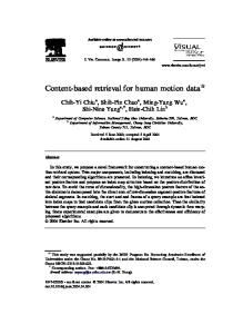
List of Figures 5.1
An example of node S’s social-tie table and its corresponding social contact graph. . . . . . . . . . . . . . . . . . . . . . . . . . . . . .
5.2
Unicast routing framework: Source node uses multi-copy routing and intermediate nodes use single-copy routing. . . . . . . . . . .
5.3
41
An example of the proposed multicast routing strategy. {D1 , D2 , D3 , D4 } form a multicast group. . . . . . . . . . . . . . . . . . . . . . . . .
5.5
35
Performance comparison of various unicast routing strategies on the San Francisco cab trace. . . . . . . . . . . . . . . . . . . . . .
5.4
32
44
Performance comparison of various multicast routing strategies on the San Francisco cab trace. . . . . . . . . . . . . . . . . . . . . .
48
5.6
Social contact graph at node s. D = {d1 , d2 } forms an anycast group. 53
5.7
Performance comparison of various anycast routing strategies on the San Francisco cab trace. . . . . . . . . . . . . . . . . . . . . .
5.8
5.9
55
Performance comparison of ASDM under different α values on the San Francisco cab trace. . . . . . . . . . . . . . . . . . . . . . . .
56
A social network graph with a fat-tailed degree distribution. . . .
57
5.10 Performance comparison of various routing strategies on the San Francisco cab trace. . . . . . . . . . . . . . . . . . . . . . . . . . .
61
5.11 Estimating parameters xmin and α of a power-law ICT distribution. 73 5.12 Performance comparison using Cabspotting trace. . . . . . . . . .
76
5.13 Delivery ratio vs message TTL in Cambridge Haggle traces. . . .
77
5.14 Delivery delay vs message TTL in Cambridge Haggle traces. . . .
77
x
6.1
Performance comparison of content retrieval schemes when content requesters and content providers belong to the same community. .
6.2
Steps in locating the content provider across communities and routing the content back to the original requester. . . . . . . . . . . .
6.3
81
85
This figure illustrates the network topology used to evaluate the proposed mechanism.
Nodes are categorized into two separate
groups featuring sub-communities, and a small subset of nodes typically traverse the divide in-between the two communities to relay information back and forth. . . . . . . . . . . . . . . . . . . . . . 6.4
Performance comparison when each node randomly requests a content within its local community. . . . . . . . . . . . . . . . . . . .
6.5
88
Performance comparison when each node randomly requests a content from a mixture of both local and foreign community. . . . . .
7.1
88
Performance comparison when each node randomly requests a content across the neighboring community. . . . . . . . . . . . . . . .
6.6
86
89
Performance comparison of different combinations of relay selection strategies and buffer management policies. . . . . . . . . . . . . .
99
7.2
Data structure to keep track of nodes and messages. . . . . . . . . 103
7.3
Performance comparison of different combinations of relay selection strategies and buffer management policies. . . . . . . . . . . . . . 112
7.4
Data structure to keep track of nodes and messages. . . . . . . . . 116
7.5
Delivery ratio vs message time-to-live in Cambridge Haggle traces. 124
7.6
Delivery delay vs buffer size in Cambridge Haggle traces. . . . . . 124
8.1
An example of caching a popular content. . . . . . . . . . . . . . 130
8.2
Performance of content retrieval with different simulation duration 133
xi
8.3
Performance of content retrieval with different cache replacement policies . . . . . . . . . . . . . . . . . . . . . . . . . . . . . . . . . 134
9.1
Performance of the content retrieval under different number of misbehaving nodes. . . . . . . . . . . . . . . . . . . . . . . . . . . . . 146
9.2
Performance of the misbehavior detection scheme under different number of misbehaving nodes. . . . . . . . . . . . . . . . . . . . . 147
xii
List of Tables 5.1
Simulation Parameters . . . . . . . . . . . . . . . . . . . . . . . .
40
5.2
Characteristics of the Cabspotting trace . . . . . . . . . . . . . .
74
5.3
Characteristics of four Cambridge Haggle traces . . . . . . . . . .
74
7.1
Notations . . . . . . . . . . . . . . . . . . . . . . . . . . . . . . .
92
7.2
Notations . . . . . . . . . . . . . . . . . . . . . . . . . . . . . . . 102
7.3
Notations . . . . . . . . . . . . . . . . . . . . . . . . . . . . . . . 114
xiii
Acknowledgments I would like to acknowledge the following people. First and foremost, my advisor Mario Gerla, for his patience and guidance. Without him, this work would not have been possible. My family for their support and trust. My current and former NRL labmates for their friendships.
xiv
Vita 2011
B.A., Computer Science Department of Computer Science University of California, Berkeley Berkeley, California
2014
M.S., Computer Science Department of Computer Science University of California, Los Angeles Los Angeles, California
2011-2016
Teaching Assistant/Graduate Student Researcher Department of Computer Science University of California, Los Angeles Los Angeles, California
Publications
T. Le and M. Gerla, “A Security Framework for Content Retrieval in DTNs”, The 12th IEEE Intl. Wireless Comm. and Mobile Computing Conf., September 2016.
T. Le, H. Kalantarian, and M. Gerla, “A Joint Relay Selection and Buffer Management Scheme for Delivery Rate Optimization in DTNs”, The 17th Intl. Symposium on a World of Wireless, Mobile, and Multimedia Networks, June 2016.
T. Le and M. Gerla, “Social-Distance Based Anycast Routing in DTNs”, The 15th IFIP Annual Mediterranean Ad Hoc Networking Workshop, June 2016. xv
T. Le and M. Gerla, “A Load Balanced Social-Tie Routing Strategy for DTNs Based on Queue Length Control”, IEEE Military Comm. Conf., October 2015.
T. Le, H. Kalantarian, and M. Gerla, “A DTN Routing and Buffer Management Strategy for Message Delivery Delay Optimization”, The 8th IFIP Wireless and Mobile Networking Conference, October 2015.
T. Le, H. Kalantarian, and M. Gerla, “A Novel Social Contact Graph Based Routing Strategy for Delay Tolerant Networks”, The 11th IEEE Intl. Wireless Communications and Mobile Computing Conf., August 2015. Best Paper Award
T. Le, H. Kalantarian, and M. Gerla, “A Two-Level Multicast Routing Strategy for DTNs”, The 14th Annual Mediterranean Ad Hoc Networking, June 2015.
T. Le, H. Kalantarian, and M. Gerla, “Socially-Aware Content Retrieval using Random Walks in DTNs”, The 9th Workshop on Autonomic Comm., June 2015.
T. Le, Y. Lu, and M. Gerla, “Social Caching and Content Retrieval in DTNs”, Intl. Conf. on Computing, Netw. and Comm., Feb. 2015. Best Paper Award
T. Le and M. Gerla, “1-to-N and N-to-1 Communication for Optical Networks”, The 8th Latin America Networking Conference, September 2014.
T. Le, V. Rabsatt, and M. Gerla, “Cognitive Routing with the ETX Metric”, The 13th Annual Mediterranean Ad Hoc Networking Workshop, June 2014.
Y. Lu, T. Le, V. Rabsatt, H. Kalantarian, and M. Gerla “Community Aware Content Retrieval in DTNs”, The 13th Ad Hoc Networking Workshop, June 2014.
xvi
CHAPTER 1 Introduction Delay Tolerant Networks (DTNs) [Fal03] are sparse mobile ad-hoc networks in which nodes connect with each other intermittently, and end-to-end communication paths are rarely available. Since DTNs allow people to communicate without network infrastructure, they are widely used in wildlife tracking [JOW02], marine monitoring [PKL07], military [LF10], and vehicular communication [OK05]. To handle the sporadic connectivity of mobile nodes in DTNs, the store-carry-andforward method is used. That is, messages are temporarily stored at a node until an appropriate communication opportunity arises. Node mobility is exploited to let mobile nodes physically carry data as relays, and forward data opportunistically when contacting others. A key challenge in DTN routing is to determine the appropriate relay selection strategy in order to minimize the number of message forwardings among nodes while maintaining a short message delivery time. Content search and retrieval is an important service in DTNs. It allows peerto-peer data sharing and access among mobile users in areas that lack a fixed communication infrastructure such as rural areas, inter-vehicle communication, and military environments. There are many applications for content retrieval in DTNs. For example, mobile users can find interesting digital content such as music and images from other network peers for entertainment purposes. Vehicles can access live traffic information to avoid traffic delay. Soldiers with wireless devices can retrieve relevant information such as terrain descriptions, weather, and intelligence information from other nodes in a battlefield.
1
Content retrieval is a defining characteristic of the Information-Centric Network (ICN), which has been drawing increased attention in both academia and industry. In ICN, users do not need to know where the content is stored, but are only interested in what the content is. Each content packet is identified by a unique name, generally drawn from a hierarchical naming scheme. The content retrieval follows the query-reply mode. A content consumer spreads the Interest packets through the network. When matching content is found either at the content provider or at the intermediate content cache server, the content data will trace its way back to the content consumer using the reverse route of the incoming Interest. Several existing ICN proposals have been studied and implemented in the Internet and Mobile Ad-Hoc Network (MANET) testbeds (e.g., CCN [JMS07], NDN [ZEB10], Vehicle-NDN [WAK12], and MANET-CCN [OLG10]). However, these are designed for connected real-time networks, and cannot be easily applied to DTN environments due to frequent partitions and intermittent connectivity among nodes. In this dissertation, we propose a secure and scalable mobile ICN architecture for content retrieval in DTNs. Given the potentially large size of mobile networks, one major design challenge of any content retrieval scheme is to locate content providers and deliver requests/contents to target nodes in a reasonable amount of time without flooding the network. Our design exploits the stable social relationships between mobile nodes for routing, caching, and placement of the content-lookup service. We rely on three key social concepts: social tie, centrality, and social level. Centrality measures the popularity of a network node, and is used to form the distributed content discovery service and the caching framework. Social level is a result of clustering centrality values, and is used to guide the forwarding of content requests to a content discovery service node. Social tie, which measures the meeting/direct delivery probability between nodes, is exploited to deliver content requests to the content provider, and content
2
data to the requester node. The material in this chapter is organized as follows. Section 1.1 introduces the key components of a content retrieval architecture. Section 1.2 presents the contributions of this dissertation. Section 1.3 provides a roadmap of the remainder of the dissertation.
1.1
Components of a Content Retrieval Architecture
There are five key components of a content retrieval framework in DTNs: a distributed content discovery service, a routing protocol for message delivery, a buffer management policy for message drop and scheduling, a caching framework to enhance the performance of data access, and a mechanism to detect malicious and selfish behaviors in the network.
1.1.1
Content Discovery Service
This component performs content lookup and reveals the identity of the content owner. In our design, we distribute the content discovery service around popular nodes (i.e., high-centrality nodes). We build the service by having each content owner advertises the compact list of content names to higher centrality nodes. We manage the content by using a low cost Bloom Filter to store the content names.
1.1.2
Routing Protocol
This component is responsible for delivering content requests (to lookup service locations and content providers) and content data (to requester nodes). There are three scenarios: (1) content is delivered to a single node (unicasting); (2) content is delivered to multiple nodes (multicasting); and (3) content is delivered to any one member in a group of nodes (anycasting). Although unicast routing
3
approaches can be used to implement group communication models, they are inefficient in terms of the transmission cost. In this dissertation, we propose different routing strategies for each of the communication models to reduce the transmission cost while achieving a high delivery ratio and low delay. Specifically, for unicast routing, we propose a forwarding metric that is based on either onehop or multi-hop delivery probabilities computed over the social contact graph. We also investigate the use of the inter-contact time (ICT) distribution to derive a relay selection metric that optimizes the delivery delay. For multicast routing, we present a dynamic multicast tree branching technique that allows routing paths to be efficiently shared among multicast destinations. Lastly, for anycast routing, we introduce an Anycast Social Distance Metric (ASDM) that balances the trade-off between a short path to the closest, single group member and a longer path to the area where many other group members reside. That is, it optimizes both the efficiency and robustness of message delivery.
1.1.3
Buffer Management Policy
This component manages the scheduling of messages, that is the order in which messages are forwarded/replicated when contact duration and forwarding bandwidth are limited. Furthermore, it is also responsible for selecting which messages to drop first when the buffer is full. In this dissertation, we develop a utility function using global network information to compute per-packet utility with respect to an optimization metric such as delivery delay or delivery ratio. Messages are then scheduled and dropped according to their utility values.
1.1.4
Caching Framework
This component is used to enhance the performance of data access. We propose a cooperative caching scheme in which popular data are cached at high-centrality
4
nodes and downstream nodes along the popular content query forwarding paths. Furthermore, neighbors of downstream nodes may also be involved for caching when there are heavy data accesses at downstream nodes. We also present a novel cache replacement policy that evicts the least popular content first when the cache is full. The content popularity is a function of both the frequency and recency of content requests. We show that this replacement policy is more superior than traditional Least Frequently Used (LFU) and Least Recently Used (LRU) policy.
1.1.5
Misbehavior Detection System
This component is responsible for detecting malicious and selfish nodes in DTNs. Since our proposed content retrieval is built upon the social-tie relationships among DTN nodes for routing and content lookup service placement, malicious nodes can launch attacks by advertising falsified social-tie information to attract and drop packets intended for other nodes, or simply disrupt and destroy the query and delivery paths. Furthermore, selfish nodes, while not seeking to attack, are unwilling to forward packets of others. Both malicious and selfish behaviors contribute to the deterioration of the content retrieval performance. To address this problem, we propose to secure both social-tie records and content delivery records during a contact between two nodes. The unforgeable social-tie records prevent malicious nodes from falsifying the social-tie information. The delivery records from which the packet forwarding ratio of a node is computed, helps detect selfish behavior. Lastly, we propose a blacklist distribution method that allows nodes to filter out misbehaving nodes from their social contact graph, effectively preventing network traffic from flowing to misbehaving nodes.
5
1.2
Contributions
In this research, we develop a secure and scalable content retrieval architecture for DTNs. This work makes the following contributions: • We show how to exploit stable social relationships among nodes to cope with the highly unstable network topology in DTNs. • We establish mathematical models to compute key social metrics, which include social tie, centrality, and social level. We then show how to build the content lookup service, caching protocol, and content forwarding protocol leveraging these social metrics. • We develop novel socially-based and ICT-based forwarding metrics for unicast, multicast, and anycast routing. • We provide theoretical frameworks for buffer management policies. • We analyze security issues of the content retrieval, and show how to use Public Key Cryptography to detect malicious and selfish nodes in the network. • We present an extensive evaluation and analysis of the architecture.
1.3
Roadmap of the Dissertation
The rest of the dissertation is organized as follows: Chapter 2 presents background materials on ICN and its recent developments. In addition, it reviews previous works related to DTN routing protocols, cooperative caching techniques, and DTN security. Chapter 3 presents the computation of key social metrics and a protocol for nodes to obtain network-wide social
6
knowledge. Chapter 4 describes the formation of the distributed content discovery service. Chapter 5 presents and evaluates the three dominant communication models (unicast, multicast, and anycast) for message delivery in DTNs. Chapter 6 outlines community-aware routing protocols for delivering content requests and content data. Chapter 7 introduces the ICT-based buffer management policy. Chapter 8 describes the cooperative caching framework. Chapter 9 discusses security issues of content retrieval in DTNs. Chapter 10 summarizes the work presented in this dissertation and briefly points out directions for future work.
7
CHAPTER 2 Background and Related Work The focus of this dissertation is on designing a secure and scalable content search and retrieval architecture in DTN networks. To facilitate the discussion of the topics presented in this dissertation, Section 2.1 presents background materials on ICN and its recent developments. Section 2.2 discusses prior works on DTN routing protocols. Related work on cooperative caching techniques are presented in Section 2.3. Finally, Section 2.4 reviews prior works on security in DTNs.
2.1
Information Centric Networks (ICNs)
ICN is an alternative approach to the architecture of IP-based computer networks. In ICN, users do not need to know where the content is stored, but are only interested in what the content is. The philosophy behind ICN is to promote content to a first-class citizen in the network. Instead of centering around IP addresses, ICN locates and routes content by unified content names, essentially decoupling content from its location. ICN differs from IP-based networks in three aspects. First, each content packet is identified by a well-defined naming scheme. Second, caching is offered through the entire network to speed up content distribution and improve network resource utilization. Third, communication follows the queryreply mode. A content consumer spreads an Interest packet through the network. The Interest packet carries a name that identifies the desired content data. When matching content is found either at the content provider or at the intermediate content cache server, the content will trace its way back to the content consumer 8
using the reverse route of the incoming Interest. Recent studies on ICN focus on high-level architectures and provide sketches of the required components. Content-Centric Network (CCN) [JMS07] and Named Data Network (NDN) [ZEB10] are two implemented proposals for the ICN concept in the Internet. Their components, including Forwarding Information Base (FIB), Pending Interest Table (PIT), and Content Store (CS) form the caching and forwarding system for the content data. Several mobile ICN architectures have also been proposed for the mobile environment, e.g., Vehicle-NDN [WAK12] for the traffic information dissemination, and MANET-CCN [OLG10] for the tactical and emergency application. However, all these architectures are designed for the connected real-time networks, and not for the disruption-tolerant mobile ICN networks. There are many potential challenges that need to be appropriately analyzed and integrated into ICN architectures for DTN networks. One prominent example is the need for delay-tolerant forwarding, a function that is increasingly important in mobile communications.
2.2
DTN Routing Protocols
DTN is a network architecture that lacks continuous network connectivity due to a number of reasons such as low density of nodes, network failures, and wireless propagation limitations. Routing protocols for DTNs exploit node mobility in order to carry messages between disconnected parts of the networks. These schemes are sometimes referred to as mobility-assisted routing that employ the store-carryand-forward method. That is, messages are temporarily stored at a node until an appropriate communication opportunity arises. Mobility-assisted routing consists of each node independently making forwarding decisions when two nodes meet. A message is forwarded to encountered nodes until it reaches the final destination.
9
A key challenge in DTN routing is to determine the appropriate relay selection strategy in order to minimize the number of message forwardings among nodes while maintaining a short message delivery time. This section reviews existing works on unicast, multicast, and anycast routing in DTNs.
2.2.1
Unicasting
Much work has been done regarding network architectures and algorithms for unicast routing in DTNs. Research on packet forwarding in DTNs originates from Epidemic routing [VB00], which floods the entire network. Spray and Wait [SPR05] is another flooding scheme but with a limited number of copies. Recent studies develop relay selection techniques to approach the performance of Epidemic routing with a lower forwarding cost. Many schemes compute the delivery probability from the encounter node to the destination before deciding whether to forward data. PROPHET [LDS03] uses the past history of encounter events to predict the probability of future encounters. LeBrun et al. [LCG05] use location information of nodes to forward data closer to the destination. Leguay et al. [LFC05b] observe that people that have similar mobility patterns are more likely to meet each other. Hence, they propose to forward data to nodes that have mobility patterns similar to the mobility pattern of the destination. Zhao et al. [ZAZ04] take a different approach by utilizing a set of special nodes called message ferries (such as unmanned aerial vehicles or ground vehicles with short range radios) to help provide communication service for other nodes through the controlled non-random movements of the ferries. Since node mobility patterns are highly volatile and hard to control, attempts at exploiting stable social network structure for data forwarding have emerged. In [MMD10], nodes are ranked using weighted social information. Messages are forwarded to the most popular nodes (highly-ranked nodes) given that popular nodes are more likely to meet other nodes in the network. The explicit friendships 10
are used to build the social relationships based on their personal communications. SimBetTS [DH09] uses egocentric betweenness centrality and social similarity to forward messages toward the node with the highest centrality, to increase the possibility of finding the optimal carrier to the final destination. BubbleRap [HCY11] combines the observed hierarchy of centrality and observed community structure with explicit labels to select the best forwarding nodes. The centrality value for each node is pre-computed using unlimited flooding. SMART [ZLF14] exploits a distributed community partitioning algorithm to divide the DTN into smaller communities. For intra-community routing, SMART uses a utility function that combines both social similarity and social centrality for relay selection. For inter-community routing, SMART chooses nodes that move frequently across communities as relays. These above works do not consider using the ICT and its distribution to optimize for relay selection. The first work that takes into account this information is [JFP04], in which the authors introduce the Minimum Expected Delay (MED) metric. MED computes the expected waiting time between pairs of nodes using the known contact schedule, and uses it to represent the delay cost for edges in the contact graph. The least delay cost routing path for each message is then computed at the source and is fixed during the entire lifetime of the message. A major drawback with MED is that it fails to exploit superior edges which become available after the route has been computed. To overcome this drawback, Jones et al. [JLS07] propose a variant of MED, which they call Minimum Estimated Expected Delay (MEED). Instead of using the known contact schedule, MEED uses the observed contact history to estimate the expected waiting time for each potential next hop. Furthermore, MEED allows message carriers other than the source node to recompute the least delay cost path to the destination of the message each time a contact arrives. This allows nodes to discover better relay nodes at a later time after message creation, thus improving the delay. Liu et al. [LW12] de-
11
fine an Expected Delay (ED) metric, which estimates the expected time it takes to deliver a message with a given remaining hop count. ED assumes that the ICTs between different node pairs are exponentially distributed and independent of each other. ED is computed considering the joint expected delay of all possible descendant forwarders in the forwarding tree. A message is forwarded/replicated to an encounter node with a smaller expected delay to the destination. In this dissertation, we propose three major unicasting strategies: 1. Social Contact Graph based Routing (SCGR) addresses the workload and throughput fairness. Unlike prior works that calculate the delivery probability from the encounter node to the destination node through direct contact, SCGR computes the delivery probability through a sequence of nodes, starting at the encounter node, on the most probable delivery path in the social contact graph. 2. Load Balanced Social-Tie Routing (LBR) addresses the load balancing issue caused by the fat-tailed distribution of connections among nodes in social networks. 3. Routing based on Expected Minimum Delay (EMD) metric deals with unforeseeable changes in the node contact topology, such as when a route suddenly becomes unavailable.
2.2.2
Multicasting
Multicast is an important group communication paradigm that enables the distribution of data to multiple receivers, such as real-time traffic information reporting, diffusion of participatory sensor data or popular content (news, software patch, etc.) over multiple devices. Multicast for DTNs has recently drawn considerable attention. Zhao et al. [ZAZ05] proposed a set of semantic models to unambiguously describe multicast in the context of DTNs. They incorporated various 12
knowledge oracles such as contact and membership into four classes of DTN routing algorithms: unicast, broadcast, tree, and group. Ye et al. [YCC06] proposed on-demand situation-aware multicast (OS-multicast) in which a node dynamically maintains a multicast tree rooted at itself to all the receivers using local knowledge of the network topology. Xi and Chuah [XC09] proposed an encounter-based multicast routing scheme (EBMR), which uses the encounter history based on PROPHET DTN unicast routing [LDS03] to disseminate a packet to the neighbors, each of which has the highest delivery predictability (within two hops) to one of the multicast receivers. In [LOL08], the throughput and delay scaling properties of multicasting in DTNs are discussed, and mobility-assisted routing is used to improve the throughput bound of wireless multicast. In [GLZ09], multicast in DTNs is considered from the social network perspective, and the social network concepts such as centrality and social community are exploited to minimize the multicast cost in terms of the number of relays used. In [MSY12], remote communication is used to assist guaranteed multicast delivery in DTNs. The problem of optimizing the remote communication cost is formalized as the demand cover problem, which is solved using a graph-indexing-based solution. In this dissertation, we propose a novel Two-Level Multicast Routing (TLMR) strategy. Unlike prior works that select relay nodes to multicast receivers based on either direct encounter probability or two-hop accumulated relay probability, and thus have a limited local view in forwarder selection, TLMR considers both short and long routing paths (two or more hops) to gain better forwarding opportunities. The two-level forwarder selection combines the benefits of a low computing overhead over short routing paths and a high delivery ratio over long (but most probable) routing paths.
13
2.2.3
Anycasting
Anycast is a network service that allows a node to send a message to any one member in a group of nodes. There are many benefits of anycast communication in DTNs. For example, anycast can be used in emergency response networks to request the help of a doctor, a fireman, or a police without knowing their IDs or accurate locations. Another example is the use of anycast in urban community networks, in which people can use the network to call for any cab. Although there is a rich literature on anycast routing in the Internet and MANETs, much less works have addressed the DTN anycast routing problems. Gong et al. [GXZ06] proposed a set of semantic models to unambiguously describe anycast in the context of DTNs. They introduced an anycast routing algorithm based on the EMDDA (Expected Multi-Destination Delay for Anycast) metric. In this algorithm, they assumed that nodes in the network are stationary, and the communication among nodes relies on a few mobile nodes that act as message carriers to deliver messages for the nodes. The algorithm computes the PED (Practical Expected Delay) values from a node to each group member, and then set EMDDA to be the minimum PED value. A mobile node then carries the message from the current node to the next hop only if the delay to get to the next hop plus the EMDDA of the next hop is smaller than the EMDDA of the current node. This relay process repeats until the message finally reaches any one of the group members. Xiao et al. [XHL10] proposed an anycast routing scheme based on the MDRA (Maximum Delivery Rate for Anycast) metric. MDRA indicates the probability that a message carrier meets a node in the anycast group, and is computed using individual meeting probabilities between a node and each group member. Based on the metric, messages are forwarded from the nodes with low MDRA values to the nodes with high MDRA values until arriving at any one of the destinations. Another anycast routing technique attempts to utilize genetic algorithms (GAs)
14
for route decisions [SG08]. The GA is applied to find the appropriate path combination to comply with the delivery needs of a group of anycast sessions simultaneously. However, this work assumes that the mobility of nodes is deterministic and known ahead of time, which is not a valid assumption for most DTNs. This dissertation presents a novel Anycast Social Distance Metric (ASDM) that differs from existing forwarding metrics in two key aspects. First, unlike existing forwarding metrics such as EMDDA and MDRA, which favor a routing path toward an anycast member with the best meeting probability, ASDM also takes into account the density of group members. More often, ASDM routes the message in the direction where most group members reside to increase the probability of meeting a group member. ASDM may also explore a sparse area with one or a few group members if these nodes have very high reachability probabilities. Thus, ASDM is more suitable for highly unpredictable networks than EMDDA and MDRA. Second, whereas existing works utilize direct encounter probabilities between a node and each group member to compute the forwarding metrics, ASDM is based on multi-hop delivery probabilities, which offer a broader view for forwarder selection.
2.3
Buffer Management Policies
Several works have investigated the issues of buffer management and message scheduling in DTNs. Zhang et al. [ZNK07] evaluated simple buffer management policies for Epidemic routing such as Drop Head (drop the oldest packet in the buffer) and Drop Tail (drop the newly received packet). They showed that Drop Head outperforms Drop Tail in terms of both delivery ratio and delay. Lindgren et al. [LP06] proposed different combinations of message drop and scheduling policies for PROPHET routing [LDS04]. They found that the best combination in terms of delivery and delay is to drop the message that has been forwarded/replicated the
15
largest number of times, and to prioritize the transmission of the message with the highest delivery predictability. Erramilli et al. [EC08] designed a queuing policy for Delegation forwarding [ECC08]. They proposed to drop the message that has been replicated the most (i.e., the message with the highest delegation number), and to prioritize the transmission of messages with a low delegation number. Similarly, Kim et al. [KY08] developed a method to compare the number of possible copies of a message. They then proposed to drop the message with the largest expected number of copies first to minimize the impact of buffer overflow. However, these works do not consider using global network information such as the number of existing copies of each message in the network and the distribution of pair-wise inter-contact times between nodes. The first work that takes into account this information is RAPID [BLV07]. RAPID handles DTN routing as a resource allocation problem that translates the routing metric into per-message utilities, which determine the order in which messages are replicated and dropped under resource constraints. However, RAPID’s utility formulation is suboptimal as it does not take into account nodes’ buffer state. Li et al. [LQJ09] introduced a buffer management policy similar to RAPID, but relaxed the assumption that messages have the same size. However, they neither addressed the message scheduling issue nor provided any experimental results to validate their scheme. Krifa et al. [KBS08] proposed a message drop policy based on per-message utilities. However, the utility is computed under the assumption of homogeneous node mobility (node pairs have the same meeting rates), which is uncommon in practice. Wang et al. [WYW15b] considered limited network bandwidth and varied message sizes. However, they still assumed a homogeneous inter-meeting rate and contact duration rate. Overall, existing works have investigated the use of inter-contact times (ICTs) to optimize buffer management strategies. However, to the best of our knowledge, they all assume exponentially distributed ICTs between mobile nodes, and
16
validate their schemes using vehicular mobility traces such as Shanghai and San Francisco taxicab traces. In this dissertation, we formulate a new buffer management strategy based on power-law distributed ICTs, while taking into account additional constraints for realistic DTNs. The scheme is validated with real-life human mobility traces. Furthermore, we revise existing buffer management policies based on exponentially distributed ICTs by introducing new models with heterogeneous node mobility and varied message sizes.
2.4
Cooperative Caching in DTNs
Cooperative caching has been studied widely in recent years. Zhuo et al. [ZLC11] proposed a social-based caching that considers the impact of the contact duration limitation on cooperative caching. Authors in [IMC10] applied a distributed caching replacement based on users’ computed policy in the absence of a central authority, and uses a voting mechanism for nodes to decide which content should be stored. In their model, mobile users are divided into several classes, such that users in the same class are statistically identical. In [GCI11], Gao et al. proposed to intentionally cache data at a set of network central locations which can be easily accessed by other nodes in the network. Wang et al. [WHK14] assumed that the popularity distribution of the network contents follows Zipf’s law. They then formulated the problem of finding the optimal cache allocation as a convex problem, and provided a binary search algorithm to find the optimal solution. Ali et al. [AR14] proposed an adaptive caching technique that uses learning automata to select nodes for caching data based on their past data forwarding ratio. Wang et al. [WWX14] presented a hierarchical cooperative caching scheme, which divides the buffer space into three components: self, friends, and strangers. This partition is intended to balance between selfishness (caching the data items according to its own preference) and unselfishness (helping other nodes to cache).
17
This dissertation proposes a social caching strategy for content retrieval that differs from previous works in two key aspects. First, we leverage the social hierarchy to determine appropriate caching locations. Popular data are cached at high social-level nodes to which most content requests are destined. To address the caching overhead at high-centrality nodes, we distribute caching data along the content request forwarding paths and around neighbors of downstream nodes. Second, regarding the cache replacement policy, we propose the Least Popular First (LPF) policy, which evicts data from the cache that is identified as least popular. This policy accounts for temporal changes in content popularity, and is more superior than Least Recently Used (LRU) and Least Frequently Used (LFU) policies, which are widely used in prior works.
2.5
Security in DTNs
In this section, we discuss previous works on detecting and mitigating the effects of malicious nodes. After that, we survey public key distribution schemes, which facilitate the use of Public Key Cryptography in DTNs.
2.5.1
Misbehavior Detection
Misbehaving nodes include selfish and malicious nodes who often drop received packets even when they have sufficient buffers. While selfish nodes are unwilling to spend their resources such as power and buffer on forwarding packets from others, malicious nodes actively seek to launch attacks either at the node level (i.e., target a specific victim) or network-wide level. Several works have been proposed to detect misbehavior in DTNs. Li et al. [LWS09] proposed to prevent an attacker from falsifying its encounter history to boost its delivery likelihood by securing the contact evidence through the usage of encounter tickets. The idea is that during a contact between two nodes, a ticket is generated and is signed by
18
two parties. When a node encounters another node, these tickets are exchanged, and are used to classify their behavior. In [LC12], a packet dropping detection technique was presented.
In this
scheme, a node keeps previous signed contact records of the buffered packets and the packets sent or received, and report them to the next contact node. A node can detect that other nodes have dropped the packets if their buffer states do not agree with the information from the records. To prevent nodes from falsifying contact records to hide the packet dropping from being detected, an honest node transmits the record summary to witness nodes. These nodes can identify the misreporting node if the summaries of contact records received from honest nodes are inconsistent with each other. A similar detection system was proposed for Vehicular Delay Tolerant Networks (VDTNs) [GSW13]. Using secure encounter records that contain contact sequence numbers and exchanged message IDs between two parties, nodes can independently detect blackhole attacks without the need to consult surrounding nodes for decision making. Another detection scheme uses trusted ferry nodes to perform intrusion detection [CYH07]. The ferries travel along fixed routes in the network, and correlate the encounter and delivery predictability information from all the nodes to identify potential malicious nodes. Similary, MUTON [RCY10b] uses ferry nodes to collect the packet delivery probability of other nodes. However, instead of cross-checking the delivery probabilities reported between a pair of nodes as in [CYH07], MUTON examines the node itself based on its recorded information of other nodes. MUTON then compares the calculated delivery probability to the claimed probability in order to determine the “sanity” of the node. Although ferry-based methods can achieve good detection performance, they may not be economical or feasible due to the requirement of additional devices (ferries) to be deployed in the network. In this dissertation, in order to prevent attackers from corrupting the social
19
contact graph, which the routing decision, caching, and lookup service placement rely upon, we seek to secure social-tie records with signatures from two encountered nodes. Furthermore, to detect the dropping of content requests and content data by misbehaving nodes, we secure packet delivery records. A suspicious node can be identified by examining the packet forwarding ratio, which is computed using the information from the delivery records. Lastly, to prevent the traffic from flowing to misbehaving nodes, we propose a mechanism to spread the blacklist of misbehaving nodes throughout the network so that nodes can filter out blacklist entries from their social contact graph. Furthermore, to prevent attackers from falsifying the blacklist, majority voting is used to determine if a blacklist is approved.
2.5.2
Public Key Distribution
Due to the lack of a fixed infrastructure in DTNs, it may not be realistic to assume that the Public Key Infrastructure (PKI) is always globally present and available. Furthermore, routing delays in DTNs prevent querying of the PKI supported by a central authority or distributed servers. Thus, the public key management becomes an open problem for DTNs. Several solutions have been proposed for public key distribution. The simplest approach is to manually preload all keys into the node during the network setup phase [RCY10a]. However, this approach is not suitable when incremental deployment of network nodes is desirable (i.e., when more nodes join the network over time). This is because the addition of new nodes whose identities are unknown during the setup phase requires their public keys to be distributed to the existing nodes, which cannot be done with preloading. Alternatively, Jia et al. [JLT12] proposed a protocol for nodes to securely exchange public keys, and then disseminate them to other network nodes. When two nodes encounter each other, they exchange their owned public keys using the two-channel cryptography technique [MS10]. The public key is transmitted using a broadband,
20
insecure wireless channel, while the verification information (such as a face-to-face conversation, voice identification, and infrared identification) is transmitted using an authenticated, narrowband manual channel. Nodes also exchange public keys that are not owned by themselves. For example, these keys are obtained from the past encounter nodes. To authenticate these keys, they proposed a key approval method, which uses majority voting among encounter nodes, who obtain the key directly from its owner to decide whether to accept the key. The distribution of public key revocation message can follow the same protocol. In this dissertation, we do not propose a new public key distribution scheme. Rather, we issue each node a private key (RK) and public key (PK) pair, and preload all public keys into the nodes during the network setup phase.
21
CHAPTER 3 Social Metrics Computation and the Formation of Network-Wide Social Knowledge The proposed content retrieval architecture is built upon three key social metrics: social-tie, centrality, and social level. Centrality is used to form the distributed content discovery service and the caching framework. Social level is used to guide the forwarding of content requests to a content discovery service node. Once the content provider ID is discovered, social tie is exploited to deliver content requests to the content provider, and content data to the requester node. In our design, each node computes the social-tie metric independently using its local observation (e.g., the history of encounter events). Knowledge of social tie can then be exchanged among nodes to enhance their network visibility, and also allows them to compute global social metrics such as centrality and social level. The material in this chapter is organized as follows. Section 3.1 describes the computation of the social-tie metric. Section 3.2 outlines a protocol for nodes to build and exchange social-tie knowledge. Section 3.3 and 3.4 respectively present the computation of centrality and social level.
3.1
Social Tie Computation
In sociological terms, social tie describes an interpersonal connection by way of friendship or acquaintance. There are many tie strength indicators: frequency, intimacy/closeness, longevity, reciprocity, recency, multiple social context, and
22
mutual confiding (trust) [DH09]. Among them, the most widely used heuristics in socially-aware networking applications are the recency and frequency of encounters [XLL13]. Two nodes are said to have a strong tie if they have met frequently in the recent past. We compute the social tie between two nodes using the history of encounter events. How much each encounter event contributes to the social-tie value is determined by a weighing function F (x), where x is the time span from the encounter event to the current time. Assume that the system time is represented by an integer, and is based on n encounter events of node i. Then, the social-tie value of node i’s relationship with node j at the current time tbase , denoted by Ri (j), is computed as: Ri (j) =
n X
F (tbase − tjk )
(3.1)
k=1
where F (x) is a weighing function, {tj1 , tj2 , · · · , tjn } are the encounter times when node i met node j, and tj1 < tj2 < · · · < tjn ≤ tbase . As an example, suppose node i met node j at times 1, 3, and 5, and that the current time (tbase ) is 10. Then, node i’s social-tie relationship with node j at tbase , denoted by Ri (j), is computed as: Ri (j) = F (10 − 1) + F (10 − 3) + F (10 − 5) = F (9) + F (7) + F (5) The weighing function F (x) essentially reflects the influence of the recency and frequency of encounter events. In order to give more weight to more recent encounter events, F (x) should be a monotonically non-increasing function. A class of functions that satisfy this condition is F (x) = ( z1 )λx , where z ≥ 2 and 0 ≤ λ ≤ 1. The control parameter λ allows a trade-off between recency and frequency in contributing to the social-tie value. As λ approaches 0, frequency contributes more than recency. On the other hand, as λ approaches 1, recency
23
has higher weight than frequency. The social-tie value is solely determined by frequency when λ = 0, and by recency when λ = 1. Following [LCK01], we set z = 2 and λ = e−4 , which have previously been shown to achieve a good trade-off between recency and frequency.
3.2
Social Knowledge Formation
In order to make an informed forwarding decision, a node needs to obtain networkwide knowledge of social-tie strength between any node pairs. This knowledge is contributed by both local observation and knowledge exchange.
3.2.1
Local Observation
Upon each encounter event, a node records the encounter node ID and the timestamp of the encounter event, and stores it in the encounter table.
Periodi-
cally, social-tie values between the current node and its direct encounters are re-computed using Eq. 3.1, where the input comes from the history of encounter events stored in the encounter table. In addition, each node maintains a social -tie-table, where each row has the following format: hpeerX, peerY, social -tie-value, timestampi Through local observation, peerX is always the current node ID. P eerY is the encounter node ID. T imestamp is the time at which the social-tie value between peerX and peerY is computed. It is the tbase variable in Eq. 3.1. As we will see next, timestamp plays an important role in knowledge exchange among nodes.
3.2.2
Knowledge Exchange
Nodes, especially those that are not socially active, tend to have limited knowledge of the social network through local observation (i.e., through direct contacts 24
with other nodes). To gain knowledge of nodes that have never met, during the encounter period, nodes can exchange and merge their local observations in the form of a social -tie-table. In the event of a merge conflict (i.e., when there are two entries with the same social -tie-value), we keep the entry with the latest timestamp. Through this process, a node can learn the social-tie values between different pairs of nodes in the network.
3.3
Centrality Computation
Centrality measures the popularity of a mobile node in a social network. It can also be regarded as a measure of how long it will take information to spread from a given node to other nodes in the network. Typically, a high-centrality node will have a low average social distance to other nodes. Thus, in its simplest form, centrality can be estimated as: PN Ci =
Ri (k) N
k=1
(3.2)
where N is the number of nodes encountered by node i, and Ri (k) is the social-tie value between node i and node k. Note that the social-tie value indicates the social distance between a pair of nodes. They have an inverse relationship. That is, the higher the social-tie value, the lower the social distance. Thus, in Eq. 3.2, a high centrality value corresponds to a high average social-tie value, which in turn implies a low average social distance. However, the average social distance metric does not consider the distribution of social-tie values. That is, a node with a single high and multiple low social-tie values can still achieve a high centrality degree, which is undesirable. For example, suppose the social-tie values between node i, j and a, b, c are as follows: Ri (a) = 30, Ri (b) = 1, Ri (c) = 2 Rj (a) = 8, Rj (b) = 10, Rj (c) = 12
25
Although node j is more central in the network than node i, node j has a lower centrality value than node i according to Eq. 3.2 (Ci = 11 > Cj = 10). To address this issue, we propose a new equation for centrality estimation, which considers both the average social-tie values and their distribution. Namely, we favor nodes with high, uniformly distributed social ties to all other nodes. For the distribution, we adopt Jain’s Fairness Index [JCH84] to evaluate the balance in the distribution of social-tie values. As in Eq. 3.3, Jain’s Fairness Index is used to determine whether users or applications are receiving a fair share of network resources. P ( ni=1 xi )2 P J (x1 , x2 , . . . , xn ) = n × ni=1 x2i
(3.3)
Jain’s equation rates the fairness of a set of values when there are n users and xi is the throughput for the ith connection. The result ranges from
1 n
(worst case)
to 1 (best case), and it is maximum when all users receive the same allocation. In our case, Jain’s Fairness Index is used to evaluate the balance of social-tie connections. The enhanced centrality metric is defined in (3.4), where N is the number of nodes encountered by node i. P PN 2 ( N k=1 Ri (k)) k=1 Ri (k) + (1 − α) Ci = α P 2 N N× N k=1 (Ri (k))
(3.4)
Here, α (set in our experiments as 0.5) is a parameter decided by the user according to the specific scenario and network conditions. For example, if there are few nodes in a large area with high mobility, a smaller α is preferred since in this scenario, the balanced connection opportunity between nodes is more important. On the other hand, if more nodes exist in a relatively small area, it is easier for nodes to meet each other, and thus a bigger α is more suitable.
26
3.4
Social Level Computation
A social level represents a group of nodes that have similar centrality (i.e., similar level of contacts with other nodes in the network). To compute social level, we use the X-means clustering algorithm [PM00] to group together nodes with similar centrality into the same cluster. A major advantage of X-means over the traditional K-means is that X-means can automatically discover the appropriate number of clusters, and runs in linear time and space in low dimensions (up to seven dimensions). For example, in our experiments, clustering the centrality values (a one-dimensional set of integers) of 10,000 nodes takes less than three seconds on an Intel Core i7 @2.9GHz. We use the existing X-means implementation that is written in standard C [PM00]. Pseudocode 1 outlines the social level computation, leveraging X-means. Pseudocode 1: Compute social level using X-means 1
clusterSet ← X -means(centralityV alues)
2
foreach clusteri ∈ clusterSet do
3
val ← computeAverageCentrality(clusteri )
4
foreach nodej ∈ clusteri do
5
nodej .socialLevel ← val
Note that in Pseudocode 1, instead of using discrete values, we directly assign average centrality values to social levels. There are two reasons behind this. First, as we will show in Chapter 5, in terms of forwarding, we only need to distinguish one social level from the other. A high average centrality value already implies a high social level. Second, assigning discrete values involves sorting the average centrality values of all clusters, which introduces unnecessary extra latency and computational overhead.
27
CHAPTER 4 Distributed Content Discovery Service A content discovery (lookup) service is the backbone of any content retrieval scheme. In our design, we distribute this service around central nodes (i.e., highcentrality nodes). Note that the set of central nodes can change over time since nodes can become socially active or inactive at different points in time. The intuition behind selecting central nodes is that central nodes tend to meet many other nodes, and thus have better knowledge of which node owns which content in the network. Furthermore, central nodes have low average social distance to other nodes, meaning that, on average, a message (e.g., a content request) can be delivered to central nodes faster than to the other nodes, thus reducing the overall latency of the content retrieval process. One important design issue with the content discovery service is content management. Any scheme that maintains and advertises a plain list of content names is inherently costly and not scalable due to its large size. Instead, we use a compact probabilistic data structure called a Bloom Filter to store the content names. The basic idea is to map a list of content names to an m-bit vector, using a set of k different hash functions, each of which maps the content name to one of the m bit vector positions. This bit vector represents our content name digest. Bloom filters are very space-efficient, and can be used to carry out content name lookups in O(1) operations. The optimal size of the Bloom Filter depends on two factors: n - the expected number of contents owned by a node, and p - the allowable false positive probability (the probability that a content is said to belong to a node
28
even though it does not). Based on [KM08], the number of bits m is computed as: m=−
n ln p (ln 2)2
Note that in (4.1), we assume that k is optimal, i.e., k =
(4.1) m n
ln 2 [KM08]. In our
experiments, we set n = 1, 000 and p = 0.05, which yields a Bloom Filter of size m = 6, 236 bits. The content discovery service is formed as follows. Each node maintains a digest table, where each row has the following format: hcontent-provider -id , content-name-digest, timestampi Here, content-name-digest is a compact representation of content names owned by the provider, and is represented using a Bloom Filter. Initially, this table is populated with a single record, which is the content-name-digest owned by the current node. Each node then actively advertises the digest table to higher centrality nodes. Upon receiving the digest table, a high-centrality node merges it into the local digest table. In the event of a merge conflict (i.e, when there are two entries with the same content-provider -id ), we keep the entry with the latest timestamp. Through this process, central nodes will eventually collect all content name digests from lower centrality nodes, and thus be able to answer different queries regarding the content provider’s identity.
29
CHAPTER 5 Routing Protocols Due to the sporadic connectivity of mobile nodes in DTNs, routing protocols often take the form of mobility-assisted routing that employs the store-carryand-forward method. In this scheme, each node independently makes forwarding decisions when two nodes meet. A message is forwarded to encountered nodes until it reaches the final destination. In the context of content retrieval, routing protocols facilitate the delivery of content requests (to lookup service locations and content providers) and content data (to requester nodes). There are three scenarios: 1) a content is delivered to a single node (unicasting); 2) a content is delivered to multiple nodes (multicasting); and 3) a content is delivered to any one member in a group of nodes (anycasting). In this chapter, we develop and evaluate several routing protocols based on the social contact graph, queue length control, and the distribution of the inter-contact times (ICTs). In addition, we outline approaches for socially-aware unicasting, multicasting, and anycasting. Unicast routing combines data “spraying” at the source node and single-copy routing at the intermediate nodes. Both multicast and anycast assume a single-copy model in which, at any point in time, there is at most one copy of the data packet per destination in the network. In multicast, all group members are destinations of the packet while in anycast, any group member is a potential destination of the packet. Thus, for example, if the multicast and anycast group are of size N , then the single-copy model results in at most N copies of the packet for the multicast and one copy for the anycast. Our objective is to
30
achieve a high delivery ratio, low delay, and low transmission cost. We discuss these protocols in a general context of message routing in DTNs, and not specific to content retrieval. As we will show in the next chapter, these protocols can be easily applied to the content request and content data forwarding in mobile ICNs. The material in this chapter is organized as follows. Section 5.1 describes the computation of multi-hop delivery probability that is used to develop the forwarding metrics for socially-aware routing protocols. Section 5.2, 5.3, and 5.4 respectively outline and evaluate social-based routing strategies for unicast, multicast, and anycast. Section 5.5 discusses inherent issues with social-based routing in resource constrained environments, and proposes a solution. Section 5.6 investigates the use of ICT distribution to optimize message delivery delay.
5.1
Multi-Hop Delivery Probability Computation
The delivery probability P (i, j) represents the likelihood that a data item buffered at node i will be delivered to node j, either through direct contact or through a sequence of two or more relays. We propose to compute the delivery probability based on the social contact graph constructed from the local social-tie table. In the social-tie table, each unique peerID represents a graph node, and each pair of peerIDs (or row) represents an undirected edge between two graph nodes. Assume there are n entries in the social-tie table. Then, the edge weight wk (i, j) of the k th entry is defined as the meeting probability between two nodes i and j relative to other pairs of nodes in the social-tie table, and is computed as: social -tie-valuerow -k wk (i, j) = Pn (5.1) k=1 social -tie-valuerow -k P where i and j are unique peerIDs, and nk=1 wk = 1. Note that we normalize the social-tie values between 0 and 1 by dividing each social-tie value by the summation of all the values in the table. The normalized social-tie values represent the edge weights in the social contact graph. As an example, Fig. 5.1 shows the 31
PeerX PeerY Social-tie S C 2 S A 3 A B 1 A D 2 B D 4 D E 3
C$
D$
2/15$
⇒
3/15$
2/15$
S$
A$ 3/15$
4/15$
1/15$
E$
B$
Figure 5.1. An example of node S’s social-tie table and its corresponding social contact graph.
social-tie table of node S after meeting and merging node A’s social-tie table, and the resulting social contact graph with the edge weights properly computed using Eq. 5.1. For simplicity, the fourth column for the timestamp is not shown, and the social-tie values are in the form of integers. In a graph, two nodes can be connected by many different paths. However, as described in the next sections, the proposed routing schemes use some form of single-copy routing, which assumes a single path between a pair of nodes. This motivates us to compute the delivery probability through the most probable path. Given a P AT Hk (i, j) between two nodes i and j, the delivery probability over the k th path can be computed as: Pk (i, j) =
Y
w(e), ∀e ∈ P AT Hk (i, j)
(5.2)
e
One way to compute the delivery probability over the most probable path is to find all the paths between i and j, compute the delivery probability through each path, and then select the maximum value. Suppose there are n paths between i and j. Then, the delivery probability through the most probable path Q(i, j) can be computed as: Q(i, j) = max {Pk (i, j), 1 ≤ k ≤ n}
(5.3)
However, this approach is computationally infeasible as finding all the paths between two nodes on an undirected graph is NP-hard. This can be proven as follows: 32
It is shown in [Hoc97] that finding the longest path between two graph nodes in an undirected graph is NP-hard. Suppose that we could find all the paths between two nodes in polynomial time. Then, by sorting the results in polynomial time, we could find the longest path, also in polynomial time. This contradiction shows that finding all the paths between two graph nodes is NP-hard. Alternatively, we propose to transform the problem of finding a path where the product of edge weights is maximized, into the problem of finding a path where the sum of edge weights is minimized. Note that the two problems are equivalent as shown below: arg max Pk (i, j) ≡ arg max log(Pk (i, j)) P AT Hk
P AT Hk
Y = arg min −log( w(e)), ∀e ∈ P AT Hk P AT Hk
= arg min P AT Hk
e
X
−log(w(e)), ∀e ∈ P AT Hk
e
A polynomial-time algorithm such as Dijkstra’s algorithm can then be used to find the least-cost path (which is the most probable path) and the corresponding delivery probability over that path. Note that the edge weights need to be transformed by negating the log values of the current edge weights. As an example, consider again the contact graph in Fig. 5.1. Suppose that S’s objective is to deliver a data item to E. Thus, upon meeting A, S is interested in computing the delivery probability from A to E. S, in turn, runs Dijkstra’s algorithm using the log-transformed edge weights (not shown on the graph). The resulting least-cost path is P AT HA→D→E with the cost (summation of logs) = (− log 2/15) + (− log 3/15) = 1.574. Note that the cost of P AT HA→B→D→E is (− log 1/15) + (− log 4/15) + (− log 3/15) = 2.449. The delivery probability is the product of non-transformed edge weights on P AT HA→D→E , which is 2/15 × 3/15 = 0.0267. For comparison, the product of non-transformed edge weights on P AT HA→B→D→E is 1/15×4/15×3/15 = 0.0036 < 0.0267. This confirms that our 33
approach correctly identifies the most probable path and computes the delivery probability over that path.
5.2
Unicast Routing Strategy
In unicast, a data item is sent from a source node to a single destination node. Although many routing schemes have been proposed, only few or none of them have addressed the fairness issue in selecting which buffered data (intended for different destinations) to forward next, upon contacting another node. An improper data selection policy can cause some destination nodes to receive disproportionately few data items. In this section, we propose a novel unicast routing strategy that balances throughput (or delivery ratio) and fairness, called Social Contact Graph based Routing (SCGR). We focus on when and where to transmit the data, which data to replicate first, and how many copies to replicate for each data packet. This section proceeds with a description of the routing protocol, followed by a performance evaluation.
5.2.1
Routing Protocol
We aim to develop a routing protocol that can deliver data items to the destination with a low delay and low overhead, while achieving a balance between throughput and fairness. To that aim, we propose to use controlled multi-copy routing at the source node and single-copy routing at intermediate nodes. Fig. 5.2 depicts our general framework. The source node S sprays three copies of data item D1 (destined to D) into the network. Each of the intermediate nodes A, B, E, and F can make at most one replication, and forward it to a node that has higher delivery probability to D than itself. All relaying nodes, including S, retain a copy of the data item until the wait timer (the duration a data item is cached at
34
a node) expires, and can perform direct transmission upon contacting D. E$
A$ D1$ D1$
B$
D$
S$ D1$
F$
Figure 5.2. Unicast routing framework: Source node uses multi-copy routing and intermediate nodes use single-copy routing.
5.2.1.1
Source node’s multi-copy routing
The source node is responsible for creating and injecting multiple replications into the network. While a larger number of replications means higher delivery rate, replicating a data item in an uncontrolled fashion can cause network congestion and wastes resources. In order to increase the utility of each replication and prevent replicating to less beneficial nodes, we propose to perform replication only if contact nodes meet the following constraints: numberOf Replica < δ P (encounterN ode, dst) > (1 + β) × bestDeliveryP robdst where P (i, j) is the multi-hop delivery probability between node i and node j. The first constraint ensures that we do not replicate endlessly and flood the network. The second constraint attempts to improve the delivery likelihood of extra replications by relaying data to a node that has better delivery probability than previous relay nodes. Initially, bestDeliveryP robdst , which is the best-so-far delivery probability to destination dst, is set to be equal to P (currentN ode, dst). Each time a data item is successfully forwarded to an encounter node subject to the above constraints, bestDeliveryP robdst is updated to P (encounterN ode, dst). 35
The factor β can be chosen to eliminate the scenario in which a data item is replicated to a series of encounter nodes with too similar delivery probabilities, and thus have small added benefits from extra replications. In our experiments, we set δ = 4 and β = 0.3. Pseudocode 2 summarizes our source node’s routing strategy. Pseudocode 2: Source node’s routing strategy 1
currentT oDst ← compDeliveryP rob(current, dst)
2
bestDeliveryP rob ← currentT oDst
3
foreach encounteri do
4
encounterT oDst ← compDeliveryP rob(encounteri , dst)
5
if (data.numOf Replica < δ)
6
&& (encounterT oDst > (1 + β) × bestDeliveryP rob) then
7
dataCopy ← replicate(data)
8
current.send(dataCopy, encounteri )
9
data.numOf Replica ← data.numOf Replica + 1 bestDeliveryP rob ← encounterT oDst
10
5.2.1.2
Intermediate node’s single-copy routing
To reduce the replication cost, intermediate nodes are allowed to make at most one replication subject to the same constraints as for the source node, but with δ = 1. It is possible for an intermediate node to hold data items destined to different nodes. Since it may not be possible to forward all data items to an encounter node within a single contact (for example, due to limited contact duration), an intermediate node needs to implement a forwarding policy that ensures fairness, while retaining high delivery throughput. A simple First-Come First-Served (FCFS) strategy is not sufficient because, for example due to node movements, the fact that data item D1 arrives at the current node before data item D2 does not neces36
sarily mean that D1 is generated and injected into the network before D2 . Thus, it may be unfair to select a data item to forward next simply based on its arrival time. Instead, we aim to ensure fairness by providing buffered data items (destined to different destinations) with an equal chance of being selected to be forwarded next. To that aim, we propose to sort arriving data into different queues corresponding to different destinations. In addition, we propose a two-level scheduler for data selection. In the first level, we use Round-Robin that selects one queue following a round-robin order. Within the candidate queue, we follow FCFS as all data items within the queue are destined to the same destination. However, a selected queue in the first level may not satisfy the forwarding constraint, i.e., the encounter node may not have a higher delivery probability toward the destination (as labeled on the queue) than the current node. Thus, instead of aborting the forwarding opportunity and hence dropping the delivery throughput, we switch to the second-level scheduler that implements priority scheduling, where the priority is defined in terms of the delivery probability to any known destination passing through an encounter node. This means that the queue with the labeled destination, toward which the encounter node has the highest delivery probability while satisfying the forwarding constraint, will be selected. Similar to the first-level scheduler, FCFS is used to select a data item within the candidate queue. An already forwarded data is removed out of the queue, but remains in a node’s caching buffer, waiting for a direct transmission opportunity with the final destination, until a wait timer expires. Note that the wait timer is used to prevent data items from being held up for too long at the source or any intermediate node. Pseudocode 3 summarizes our intermediate node’s routing strategy. Lastly, note that a node can hold its self-owned data and data arriving from other nodes. That is, a node can serve the role of a source node and an intermediate node simultaneously. In this case, regarding data selection, we give higher priority to self-owned data. Upon contacting a node, the current node will first
37
Pseudocode 3: Intermediate node’s routing strategy 1
foreach encounteri do
2
f orwardingF lag ← f alse
3
queue ← roundRobinSelection()
4
if compDeliveryP rob(encounteri , queue.dst) > (1 + β) × compDeliveryP rob(current, queue.dst) then
5 6
f orwardingF lag ← true else
7
queue ← prioritySelection()
8
if compDeliveryP rob(encounteri , queue.dst) > (1 + β) × compDeliveryP rob(current, queue.dst) then
9
f orwardingF lag ← true
10
if f orwardingF lag = true then
11
data ← F CF SSelection(queue)
12
dataCopy ← replicate(data)
13
current.send(dataCopy, encounteri )
14
queue.remove(data)
38
pick self-owned data to forward next, subject to the source node’s forwarding constraints. If the forwarding constraints are not met, the current node will select data items (arriving from other nodes) following intermediate node’s single-copy routing strategy.
5.2.2
Performance Evaluation
In this subsection, we evaluate the performance of the proposed SCGR scheme in a packet-level simulation, using a real-world mobility trace. We first describe the simulation setup, followed by the metrics used and the results.
5.2.2.1
Simulation Setup
We implement the proposed routing protocol using the NS-3.19 network simulator. DTN nodes advertise Hello messages every 100ms. In order to test the bottom line of the performance, we assume that each source node owns a unique data item. We also assume that all data is of the same size (1MB) to ensure that the measurement is not affected by variations in data size. We use the IEEE 802.11g wireless channel model and the PHY/MAC parameters as listed in Table 5.1. To obtain meaningful results, we use the real-life mobility trace of San Francisco’s taxi cabs [cab]. This data set consists of GPS coordinates of 483 cabs, collected over a period of three consecutive weeks. For our studies, we pick an NS-3 compatible trace file from downtown San Francisco (area dimensions: 5,700m x 6,600m) with 116 cabs, tracked over a period of one hour [Lak]. We fix the broadcast range of each moving object to 300m, which is typical in a vehicular ad hoc network (VANET) setting [Al 14]. We evaluate SCGR against three existing DTN routing schemes: PROPHET [LDS03], BubbleRap [HCY11], and Epidemic routing [VB00]. PROPHET is a utility-based routing protocol that uses the past history of encounter events to
39
Table 5.1. Simulation Parameters Parameter RxNoiseFigure TxPowerLevels TxPowerStart/TxPowerEnd m channelStartingFrequency TxGain/RxGain EnergyDetectionThreshold CcaModelThreshold RTSThreshold CWMin CWMax ShortEntryLimit LongEntryLimit SlotTime SIFS
Value 7 1 12.5 dBm 2407 MHz 1.0 -74.5 dBm -77.5 dBm 0B 15 1023 7 7 20 µs 20 µs
forward data to nodes with higher delivery predictability to the destination. BubbleRap is a community-based algorithm that routes data based on rankings calculated from social centrality. Lastly, Epidemic routing is a flooding-based protocol, which has a delivery ratio and delay that approach the theoretical maximum, but also has the highest delivery cost. In our experiments, each node sends a unique data item to a random destination in the network. For statistical convergence, we repeat each simulation 20 times.
5.2.2.2
Evaluation Metrics
We use the following metrics for evaluation: • Delivery ratio: the proportion of data items that have been delivered out of the total unique data items created. • Average delay: the average interval of time for each data item to be delivered from the source to the destination. • Total cost: the total number of data replications in the network.
40
0.7
2500
Epidemic SCGR PROPHET BubbleRap
2000 Average delay (sec)
Delivery ratio
0.5 0.4 0.3 0.2
12000
Epidemic SCGR PROPHET BubbleRap
10000
1000
2000
0.1
75
150
450 750 1500 Duration (sec)
2250
3000
(a) Delivery ratio
3600
6000
4000
500
0 15
Epidemic SCGR PROPHET BubbleRap
8000
1500
Total cost
0.6
0 15
75
150
450 750 1500 Duration (sec)
2250
3000
(b) Average delay
3600
0 15
75
150
450 750 1500 Duration (sec)
2250
3000
3600
(c) Total cost
Figure 5.3. Performance comparison of various unicast routing strategies on the San Francisco cab trace.
5.2.2.3
Comparative Results
Fig. 5.3 shows the performance of Epidemic, PROPHET, BubbleRap, and our proposed SCGR scheme. The delivery ratio is compared in Fig. 5.3a. As we increase the simulation time from 15 seconds to 3,600 seconds, the delivery ratio of all schemes is improved. As expected, Epidemic has the highest delivery ratio. By using a flooding method, Epidemic can deliver data items to even remote nodes with a high probability. SCGR outperforms PROPHET by about 7% and BubbleRap by 10%. BubbleRap performs the worst perhaps because it is impacted by the weak community structure in the San Francisco cab trace. Recall that BubbleRap is a community-based algorithm, which makes data forwarding decision heavily based on the community structure of the network. In terms of the average delay as shown in Fig. 5.3b, SCGR has a delay as low as Epidemic, which is much lower than the other two strategies. Lastly, the total cost is compared in Fig. 5.3c. Epidemic has the highest cost as it floods packets to every network node. The cost of PROPHET is the second highest, as each node (regardless of whether it is a source or intermediate node) uses multi-copy routing to replicate data items to encounter nodes with higher delivery predictability. SCGR has a lower cost than PROPHET due to the single-copy routing strategy implemented at the intermediate nodes. BubbleRap has the lowest cost because of its self-
41
limited replication strategy that deletes data items from the original carrier as soon as they are delivered to the community of the target destination node.
5.3
Multicast Routing Strategy
In multicast, a data item is sent from a source node to an arbitrary set of destination nodes. Although multicasting can be implemented by sending a separate copy of data via DTN unicast to each multicast receiver, such an approach is inefficient and can consume lots of network resources. Furthermore, multicast approaches that are proposed for the Internet or well-connected MANETs cannot be directly applied to DTN environments due to frequent partitions and intermittent connectivity among nodes. Thus, we are motivated to develop an efficient multicast routing scheme for DTNs. In this section, we propose a novel Two-Level Multicast Routing (TLMR) strategy. Our scheme is based on the single copy model in which, at any point in time, there is at most one copy of the data packet for each multicast destination in the network. We focus on reducing the transmission cost by bundling as many multicast receivers as possible into a single copy, and forwarding it to an encounter node with high delivery probabilities to those multicast receivers. This allows routing paths to be efficiently shared among multiple destinations. At the same time, we optimize both the delivery rate and computing resource by alternating between using the one-hop delivery probability (which is less accurate, but can be quickly computed) and multi-hop delivery probability (which is more accurate, but takes a longer time to compute) in forwarder selection. This section proceeds with a description of the routing protocol, followed by a performance evaluation.
42
5.3.1
Routing Protocol
We consider a single-copy model in which, at any point in time, there is at most one copy of the data packet per multicast destination in the network. Furthermore, copies that are intended for different destinations can be scattered at different nodes. Suppose that there are D multicast receivers. Our key idea for multicast routing is to have the source node S delegate a subset Q ⊆ D to an encounter node E subject to the following forwarding constraint: ∀x ∈ Q, P (E, x) > (1 + β) · P (S, x)
(5.4)
where P (i, j) is the delivery probability from node i to node j, and β > 0 (set in our experiments as 0.3) is used to avoid replicating to an encounter node with a too similar delivery probability. Subsequently, each intermediate node follows the same strategy on a smaller subset, until the multicast data is delivered to all multicast members. For example, in Fig. 5.4, at time t1 , S encounters two nodes n1 and n3 . After exchanging and merging social-tie tables, S computes the delivery probabilities from n1 and n3 to the multicast members. S then finds that n1 has a higher delivery probability to D1 than itself, and n3 has a higher delivery probability to D2 , D3 , and D4 than itself. Thus, S creates two copies of the packet. One copy is sent to n1 with a header that includes D1 in the final destination set. The other copy is sent to n3 with a header that includes D2 , D3 , and D4 in the final destination set. To obey the single-copy model, S removes D1 , D2 , D3 , and D4 out of its destination set. Since the destination set at S becomes empty, S removes the data from its caching buffer. At time t2 , n1 meets n2 , and n3 meets D2 and n4 . Since n2 has a higher delivery probability to D1 than n1 , n1 forwards its only copy to n2 . Similarly, n3 duplicates two copies, one with a header that includes D2 and D3 to be sent to D2 , and the other with a header that includes D4 to be sent to n4 . At time t3 , direct transmissions are performed upon meeting multicast members, ignoring the delivery probability comparison 43
step. n2$
D1$
n2$
n1$
D1$
n2$
n1$
S
D2$
n3$
D3$
n1$
S
D2$
n3$
n4$
D3$
S
D2$
n3$
n4$ D4$
t1$
D1$
n4$ D4$
t2$
D3$
D4$
t3$
Figure 5.4. An example of the proposed multicast routing strategy. {D1 , D2 , D3 , D4 } form a multicast group.
Next, we propose a two-level strategy for electing a subset of multicast members to be forwarded to an encounter node. Both levels correspond to different ways of computing the delivery probability. In the first level, we use the direct (one-hop) delivery probability, which can be inferred from the social-tie strength between a pair of nodes. Typically, a higher social-tie strength implies a higher delivery probability between two nodes. Thus, we replace P (i, j) with Ri (j) in the forwarding constraint, where Ri (j) is the social-tie strength between i and j as defined in Eq. 3.1. The benefit of using Ri (j) is that it can be computed quickly, with little overhead. However, Ri (j) may not be the best indicator for the delivery probability toward a final destination, as it only considers a one-hop relay, which has a very limited local view. For example, if the current node A and its encounter node B have not met any multicast member dx , then RA (dx ) = 0, and RB (dx ) = 0. Consequently, A cannot determine whether B is a good relay, even though B may often meet other nodes that have high delivery probabilities to multicast destinations. To resolve this issue, we propose a second-level strategy that uses the multi-hop delivery probability (as computed in Section 5.1) for forwarder selection. The multi-hop delivery probability takes into account a broader view of the network, thus allowing a node to make a more informed forwarding decision. Considering again our previous example, using the multi-hop delivery
44
probability, A will see that B can reach intermediate nodes that have strong connections to multicast members. Thus, A will choose B as a relay node, which is a desired behavior. Pseudocode 4: A two-level multicast routing strategy 1 2 3
foreach encounteri do foreach dj ∈ data.destSet do if socialT ie(encounteri , dj ) > (1 + β) × socialT ie(current, dj ) then
4
dataCopyi .addT oDestSet(dj )
5
data.removeF romDestSet(dj )
6 7 8 9 10 11
if dataCopyi .destSet 6= N U LL then current.send(dataCopyi , encounteri ) else Q ← pickLRandomN odes(data.destSet) foreach dj ∈ Q do if compM ultihopP rob(encounteri , dj ) > (1 + β) × compM ultihopP rob(current, dj ) then
12
dataCopyi .addT oDestSet(dj )
13
data.removeF romDestSet(dj )
14 15
if dataCopyi .destSet 6= N U LL then current.send(dataCopyi , encounteri )
16
if data.destSet = N U LL then
17
current.remove(data)
However, the computation of the multi-hop delivery probability is non-trivial (for example, in the order of O(|E| + |V |log|V |) if using Dijkstra’s algorithm, where |V | is the number of vertices and |E| is the number of edges). Thus, it is not practical to apply this multi-hop delivery probability computation to all multicast members if the multicast group size is large. Instead, at the second level, we propose to perform only L multi-hop delivery probability computations, where the L multicast destinations are chosen randomly from the multicast group. 45
Typically, the choice of L depends on the computing resource of a mobile node. In our experiments, we set L = 5. Pseudocode 4 summarizes our multicast routing strategy. When a node must deliver a packet to L or fewer destinations, the second-level forwarding strategy is exclusively used (not shown in the pseudocode). Otherwise, a two-level strategy is used: routing is initially achieved using the first level, switching to the second-level strategy when no multicast members satisfy the forwarding constraint.
5.3.2
Performance Evaluation
In this subsection, we evaluate the performance of the proposed TLMR scheme in a packet-level simulation, using a real-world mobility trace. We first describe the simulation setup, followed by the metrics used and the results.
5.3.2.1
Simulation Setup
We implement the proposed routing protocol in NS-3.19. We use the same trace and network parameters as in the previous section. In the experiments, we randomly set one of the 116 nodes as the source, and choose other nodes as multicast destinations. We vary the number of destinations from 2 to 30. The source node transmits a data packet of size 1MB after 1,000 seconds of the warming-up period. Each simulation has a length of one hour. For statistical convergence, we repeat each simulation 20 times. We evaluate TLMR against two existing DTN multicast routing schemes: single-copy EBMR [XC09] and multiple-copy Epidemic routing [VB00]. EBMR performs tree branching dynamically in a manner similar to our level-1 routing strategy. However, it is based on PROPHET DTN unicast routing [LDS04], which considers the delivery probability to multicast receivers within two hops. Epidemic routing is a flooding-based protocol. The multicast implementation of Epidemic
46
routing creates a copy of the data, bundles all multicast destinations into the copy, and forwards the packet to the encounter node. Epidemic routing typically has the highest delivery ratio and lowest delay, but also has the highest delivery cost.
5.3.2.2
Evaluation Metrics
We use the following metrics for evaluation: • Delivery ratio: the proportion of destinations that receive the data item out of the total number of intended destinations. • Average delay: the average interval of time required for a multicast destination to receive the data item. • Average cost: the average number of relays required for a multicast destination to receive the data item.
5.3.2.3
Comparative Results
Fig. 5.5 shows the performance of Epidemic, EBMR, and our proposed TLMR scheme. The delivery ratio is compared in Fig. 5.5a. As expected, Epidemic has the highest delivery ratio. By using a flooding method, Epidemic has a higher chance to successfully deliver a data item to hard-to-reach destinations compared to other multicast approaches. TLMR outperforms EBMR by about 7% on average. Clearly, TLMR’s second-level relay selection strategy that considers multihop forwarding opportunities, allows the data item to take a highly probable path to reach the destination before the simulation ends, thus improving the delivery ratio. Furthermore, we note that the delivery ratio fluctuates as we vary the number of receivers. This is because multicast destinations are selected randomly during each simulation. Some destinations are very difficult to reach within the simulation time, even using a flooding-based strategy such as Epidemic routing.
47
Thus, the selection of more remote destinations in a particular run will lower the delivery ratios of all three schemes compared to other runs. In terms of the average delay as shown in Fig. 5.5b, Epidemic has the smallest average delay as a result of its flooding-based approach. TLMR has a lower delay than EBMR because TLMR’s forwarding policy considers long routing paths that may generate faster routes to multicast destinations. Due to random selections of multicast receivers for each run, and because some destinations take a longer time to reach than the others, it is expected to see the delay fluctuates as the multicast group size is varied. Lastly, average cost is compared in Fig. 5.5c. Epidemic has the highest cost as it floods the packet to every network node. TLMR has a slightly higher cost than EBMR because TLMR considers using long but fast paths for multicast routing. However, TLMR has a higher delivery ratio and lower average delay. 1
6
2500
0.9
5
0.8
2000
0.6 0.5 0.4 0.3 0.2
0 2
5
10 15 20 Number of receivers
25
(a) Delivery ratio
1500
1000
30
3
2
500
Epidemic TLMR EBMR
0.1
4 Average cost
Average delay (sec)
Delivery ratio
0.7
0 2
1
Epidemic TLMR EBMR 5
10 15 20 Number of receivers
25
(b) Average delay
30
0 2
Epidemic TLMR EBMR 5
10 15 20 Number of receivers
25
30
(c) Average cost
Figure 5.5. Performance comparison of various multicast routing strategies on the San Francisco cab trace.
5.4
Anycast Routing Strategy
In anycast, a message is sent from a source node to any one member in a group of nodes. Although many anycast routing protocols have been proposed in the Internet and MANETs, they cannot be easily applied to DTNs due to the lack of
48
stable end-to-end paths to a destination group member. Furthermore, in traditional DTN unicast routing, the destination of a message is fixed at the time of creation. By contrast, the destination can change dynamically in anycast routing according to the movement of nodes. As a result, anycast routing in DTNs is a particularly challenging problem. In this section, we focus on developing an anycast routing scheme that is both robust and efficient (e.g, having a high delivery probability and short delay). The scheme is based on the single-copy model in which there is at most one copy of the message in the network. To cope with the highly volatile node mobility, we exploit the stable social network structure for message forwarding. We propose a novel forwarding metric called Anycast Social Distance Metric (ASDM), which is a function of multi-hop social distances to anycast group members. The forwarding decision based on ASDM considers the trade-off between a short path to the closest, single group member (i.e., short social distance) and a longer path to the area where many other group members reside. While the former can shorten the delivery delay, it is less robust than the latter, especially when the nearest node is socially isolated from other group members, and it may often leave or move to another location in a dynamic network. Note that the robustness of the latter choice comes from the intuition that a node is more likely to encounter a particular group member if it is closer to many group members. This section proceeds with the development of the anycast delivery probability metric, followed by a description of the routing protocol and a performance evaluation.
5.4.1
Anycast Delivery Probability Metric
In this subsection, we introduce two metrics based on the social-tie information between nodes to evaluate the chance that a node can successfully deliver a packet to any one member of an anycast group either through direct contact or through a sequence of two or more relays. We consider an anycast group D of size n, in 49
which D = {d1 , d2 , · · · , dn }.
5.4.1.1
Anycast Direct Encounter Metric (ADEM)
ADEM is defined as the probability of directly encountering at least one node in the anycast group. We compute this metric by first normalizing the social-tie values between 0 and 1. Let M (i, j) denote the meeting probability between two nodes i and j. Then, based on our earlier analysis from Section 5.1, M (i, j) is the normalized social-tie value between i and j. That is, M (i, j) = w(i, j), where w(i, j) is computed as in Eq. 5.1. The probability that a node x meets any node in set D can be computed as: ADEM (x, D) = 1 −
Y
(1 − M (x, d))
(5.5)
d∈D
where
Q
d∈D (1−M (x, d))
is the probability that x does not meet all members of the
group. A metric similar to ADEM has been proposed in [XHL10]. Yet, ADEM differs in terms of how M (x, d) is computed. In this subsection, we introduce ADEM primarily for comparison purposes against Anycast Social-Distance Metric, which we describe next.
5.4.1.2
Anycast Social-Distance Metric (ASDM)
ASDM is defined as the probability of successfully delivering a packet to any members of an anycast group based on the social distances to members of the group. The social distance SD(x, di ) from a node x to a member di ∈ D is formulated as: SD(x, di ) = 1 − P (x, di )
(5.6)
where P (x, di ) is the multi-hop delivery probability over the most probable path from x to di (see Subsection III-C). This formulation favors an encounter node x with a high multi-hop delivery probability to di (i.e., a small social distance 50
toward the destination). Intuitively, in order to increase the chance of reaching any group member in an unpredictable network, we should favor a relay node that is “socially” close to the network area where more group members reside. Inspired from [LNK05], we model ASDM based on the individual social distance to each group member as shown below: ASDM (x, D) ∝
1 SD(x, d)α d∈D
X
(5.7)
where 0 ≤ SD(x, d) ≤ 1 and α > 0. The control parameter α determines the balance between forwarding in the direction where most group members reside and forwarding toward a few close members. While a small value of α favors the former direction, a larger value of α prefers the latter direction. Depending on the network characteristic, α should be tuned carefully so that anycast packet can be forwarded in the direction that has a high chance to meet a group member with a short delay. In our experiments, we found that α = 1.5 allows for reasonable results. The value of ASDM (x, D) ranges from 0 to ∞, and it is ∞ when x is an anycast group member. As an example, consider an anycast group D = {d1 , d2 , d3 , d4 }. Suppose that the current node with the anycast packet meets two relay nodes u and v that have the multi-hop delivery probabilities to the four group members as follows: P (u, di ) = [0.2, 0.4, 0.3, 0.1] and P (v, di ) = [0.1, 0.05, 0.1, 0.5]. The corresponding social distances are SD(u, di ) = [0.8, 0.6, 0.7, 0.9] and SD(v, di ) = [0.9, 0.95, 0.9, 0.5]. As we can see, u is socially closer to d1 , d2 , and d3 than v, whereas v is closer to d4 than u. Also, note that the shortest distance between a relay to group D is SD(v, d4 ) = 0.5. Since SD(v, d4 ) is not significantly shorter than min {SD(u, di ), 1 ≤ i ≤ 4}, ASDM metric (with α = 1.5) will prefer u over v as a relay node (ASDM (u, D) = 6.43 > ASDM (v, D) = 6.25). That is, ASDM will select the direction toward an area where most group members reside. Note that if SD(v, d4 ) becomes further smaller (i.e., when P (v, d4 ) ≥ 0.6), ASDM will 51
instead favor v over u as a relay node. This decision is justifiable since the value of SD(v, d4 ) is now in a safe range, in which we have a certain confidence in reaching the closest anycast member d4 despite that it may be socially isolated from other group members. Compared to ADEM metric, ASDM is more conservative. That is, ASDM is less attracted toward the closest, single member than ADEM. Rather, ASDM attempts to balance between moving toward an area with many group members (which is more robust) and moving toward a few closer members (which is more efficient). Furthermore, by considering long routing paths with multi-hop delivery probabilities, ASDM has a broader view for forwarder selection than ADEM, which only considers one-hop routing paths through direct meeting between a relay node and a group member. To see the benefit of using multi-hop delivery probabilities in the formulation of an anycast routing metric, considering the following example. Suppose that the source node s meets node x, and it aims to deliver a packet to an anycast group D = {d1 , d2 }. Fig. 5.6 shows the contact graph constructed by s. Node x has no edges to anycast members since it has not encountered any group members in the past. Thus, ADEM (x, D) = 0. Consequently, s mistakenly identifies x as a bad relay node, even though x may often meet v who has strong connections to anycast members. In contrast, ASDM takes into account a broader view of the network. ASDM uses multi-hop delivery probabilities from x to d1 and d2 in computing social distances, which results in ASDM (x, D) > 0. As a result, s correctly identifies x as closer to the anycast group, and thus selects x as a next relay node, which is a desired behavior.
52
u$
s$
d1$
x$ v$
d2$
Figure 5.6. Social contact graph at node s. D = {d1 , d2 } forms an anycast group.
5.4.2
Performance Evaluation
In this subsection, we evaluate the performance of the proposed ASDM-based routing scheme in a packet-level simulation, using a real-world mobility trace. We first describe the simulation setup, followed by the metrics used and the results.
5.4.2.1
Simulation Setup
We implement the proposed routing protocol in NS-3.19. We use the same trace and network parameters as in Section 5.2. In our experiments, we select 5 random nodes as the destination anycast group members. Every other node acts as the anycast source, which transmits a unique data packet of size 1MB after 1,000 seconds of the warming-up period. For statistical convergence, we repeat each simulation 20 times with different random seeds. We evaluate ASDM (where α = 1.5) against ADEM, UBA, and Epidemic routing [VB00]. ADEM and UBA were introduced in Section III-D and III-E, respectively. ADEM forwards the message based on the probability of directly encountering any one group member. UBA extends the unicast protocol, and routes the message to a fixed destination, to which the source node has the highest multi-hop delivery probability at the time of message creation. Epidemic routing is a flooding-based protocol, which has a delivery ratio and delay that approach the theoretical maximum, but also has the highest delivery cost.
53
5.4.2.2
Evaluation Metrics
We use the following metrics for evaluation: • Delivery ratio: the proportion of unique packets that are received by an anycast group out of the total number of unique packets generated. • Average delay: the average interval of time required for an anycast group to receive the data item. • Average cost: the average number of relays required for an anycast group to receive the data item.
5.4.2.3
Comparative Results
Fig. 5.7 shows the performance of Epidemic, ADEM, UBA, and our proposed ASDM scheme. The delivery ratio is compared in Fig. 5.7a. As we increase the simulation time from 1,000 seconds (the warming-up period) to 3,600 seconds, the delivery ratio of all schemes is improved. As expected, Epidemic has the highest delivery ratio. By using a flooding method, Epidemic has a high chance to successfully deliver a data item to an anycast group, even when the group is comprised of hard-to-reach members. ASDM outperforms ADEM by more than 10%. The improvement of ASDM over ADEM is a result of two factors. First, the use of multi-hop delivery probabilities generates more path choices to reach a group member than the direct (one-hop) delivery probabilities. Second, from this pool of available paths, the function of social distances to group members allows the selection of the most probable path to reach at least one group member. Lastly, UBA performs the worst because the best group member at the time of message creation is likely to change over time, and thus, unicasting to this member is not guaranteed to be successful within the simulation time. In terms of the average delay as shown in Fig. 5.7b, Epidemic has the smallest 54
average delay as a result of its flooding-based approach. ASDM has a lower delay than ADEM and UBA. This is because ASDM considers multi-hop forwarding opportunities, which enable a packet to travel through a fast route to an anycast group member. Furthermore, a well-tuned parameter α in ASDM function, while favoring density of group members over proximity, can drive a packet to the nearest group member if it possesses a high successful delivery probability. This has the effect of reducing the routing delay. Lastly, average cost is compared in Fig. 5.7c. Epidemic has the highest cost as it floods the packet to every network node. The cost of UBA is the second highest as UBA is vulnerable to the movement of the best node that is selected at the time of message creation. ADEM has a lower cost than UBA because ADEM takes a group-based view for anycast routing, and therefore is not vulnerable to the movement of a particular group member. Finally, ASDM has a lower cost than ADEM because the delivery probability of ASDM is more stable than ADEM, thus making ASDM less vulnerable to the movement of the entire group. Note that the stability of ASDM is due to its consideration of a broad network view based on multi-hop delivery probabilities and the density of group members.
0.8
2500
ASDM ADEM UBA Epidemic
2000 Average delay (sec)
Delivery ratio
0.7 0.6 0.5 0.4 0.3 0.2
6
ASDM ADEM UBA Epidemic
5
ASDM ADEM UBA Epidemic
4 Average cost
1 0.9
1500
1000
3
2
500
1
0.1 0 1000
1500
2000 2500 Duration (sec)
3000
(a) Delivery ratio
3600
0 1000
1500
2000 2500 Duration (sec)
3000
(b) Average delay
3600
0 1000
1500
2000 2500 Duration (sec)
3000
3600
(c) Average cost
Figure 5.7. Performance comparison of various anycast routing strategies on the San Francisco cab trace.
55
5.4.2.4
Effect of Values of α on ASDM Routing Strategy
In this subsection, we evaluate the performance of ASDM with different α values. Recall from Subsection III-D that small values of α drive packets in the direction where most group members reside, whereas for large values of α, packets are more attracted toward the close members. The results are plotted in Fig. 5.8. We find that increasing α improves the delay and cost at the expense of lower delivery ratio. This implies that in DTN networks characterized by highly volatile node movements, choosing a (long) routing path over which many members are accessible will result in a higher delivery ratio than a path to a closer, single member. Furthermore, we observe that an α value of 1.5 allows a reasonable trade-off among delivery ratio, delay, and transmission cost.
0.8
2500
α=0.5 α=1.0 α=1.5 α=2.0
2000 Average delay (sec)
Delivery ratio
0.7 0.6 0.5 0.4 0.3 0.2
6
α=0.5 α=1.0 α=1.5 α=2.0
5
α=0.5 α=1.0 α=1.5 α=2.0
4 Average cost
1 0.9
1500
1000
3
2
500
1
0.1 0 1000
1500
2000 2500 Duration (sec)
3000
(a) Delivery ratio
3600
0 1000
1500
2000 2500 Duration (sec)
3000
(b) Average delay
3600
0 1000
1500
2000 2500 Duration (sec)
3000
3600
(c) Average cost
Figure 5.8. Performance comparison of ASDM under different α values on the San Francisco cab trace.
5.5
Routing Based on Queue Length Control
Social-based routing protocols such as PROPHET [LDS03], SimBetTS [DH09], BubbleRap [HCY11], and those proposed in Section 5.2 - 5.4 tend to select the next hop node that is the most “popular” or has the highest delivery predictability with the destination. In complex/social networks where connections among nodes follow a fat-tailed distribution (see Fig. 5.9), this strategy will guide the message
56
Figure 5.9. A social network graph with a fat-tailed degree distribution.
toward a few highly connected nodes. Under a constrained buffer and battery capacity, high-degree nodes will become network bottlenecks. As a consequence, messages will be dropped more often and message loss becomes inevitable as the battery power drains quickly. This greatly affects the overall delivery ratio. In this section, we propose Load Balanced Social-Tie Routing (LBR). LBR selects relay nodes based on the combination of social-tie delivery probability and queue length control (back pressure control) in order to spread traffic more evenly across the network, and thus avoiding frequent message drops due to congested buffer space at highly-connected nodes. This section proceeds with a description of the routing protocol, followed by a performance evaluation.
5.5.1
Routing Protocol
We use a single-copy model in which, at any point in time, there is at most one copy of the message in the network. To achieve a high delivery ratio and low cost, we favor nodes that are good candidates to deliver the message successfully to their destination. In our routing strategy, a message carrier node i will forward the message to an encountered node j if and only if j has a higher social tie with the destination k than i. That is, the following condition must hold: Rj (k) > Ri (k)
57
(5.8)
In some cases, node i and its encounters may not have any social tie with the target destination k because, for example, they have never come into contact with k. Thus, the relay selection based on (5.8) can cause the message to get stuck in a node’s queue infinitely. To address this problem, we propose to forward a message to an encountered node that has a higher potential to deliver the message to any node. That is, X
Rj (x) >
x∈Nj
X
Ri (x)
(5.9)
x∈Ni
where Ni and Nj are the set of nodes encountered by i and j, respectively. In summary, to optimize the delivery ratio and cost, node i only forwards a message intended for k to j if and only if any of the following conditions is met: R �j (k) > Ri (k) � � � P P (5.10) Rj (x) > Ri (x) ∧ Ri (k) + Rj (k) = 0 x∈Nj
x∈Ni
However, this heuristic, just like any other existing heuristics, does not address the load balancing problem. In fact, it still biases toward high-degree nodes. To achieve load balancing, we use a queue length control mechanism such that traffic is temporarily diverted away from congested nodes (i.e., high-degree nodes). In this mechanism, nodes can only forward packets to nodes of similar or smaller queue length. That is, a congested node is allowed to forward packets to a less congested node, but not the other way around. The intuition behind this scheme is as follows: The queue length reflects a node’s connectivity. A highly connected node tends to receive lots of packets, and thus its queue length grows larger than others. By enforcing nodes to forward packets only to nodes of similar or smaller queue length, we can effectively divert traffic away from congested nodes, while allowing nodes to explore alternative paths. Over time, as packets flow out of congested nodes, their queue length becomes smaller, and the control mechanism will dynamically enable the traffic to flow into these nodes again. As we will show in the evaluation, this queue length control strategy results in a more balanced 58
load distribution without compromising delivery ratio and cost. With the queue length control, a node i will forward a message intended for k to j if any of the following conditions is met:
� � R (k) > R (k) ∧ (QLj ≤ QLi ) i � j � � � P P Rj (x) > Ri (x) ∧ (Ri (k) + Rj (k)) = 0 ∧ (QLj ≤ QLi ) x∈Nj
(5.11)
x∈Ni
where QLi and QLj are the queue lengths of node i and j, respectively.
5.5.2
Performance Evaluation
In this subsection, we evaluate the performance of our proposed LBR scheme in a packet-level simulation, using a real-world mobility trace. We first describe the simulation setup, followed by the metrics used and the results.
5.5.2.1
Simulation Setup
We implement the proposed routing protocol using the NS-3.19 network simulator. To obtain meaningful results, we use the real-life mobility trace of San Francisco’s taxi cabs [cab]. This data set consists of GPS coordinates of 483 cabs, collected over a period of three consecutive weeks. For our studies, we select an NS-3 compatible trace file from downtown San Francisco (area dimensions: 5,700m x 6,600m) with 116 cabs, tracked over a period of one hour [Lak]. Vehicles advertise Hello messages every 100ms [EWK09]. The broadcast range of each vehicle is fixed to 300m, which is typical in a vehicular ad hoc network (VANET) setting [Al 14]. We evaluate the performance of LBR against the following algorithms: • Epidemic routing [VB00] is a flooding-based multi-copy routing algorithm. It is optimal in terms of delivery ratio, but is very inefficient in 59
terms of cost (the number of forwardings). Furthermore, Epidemic routing is expected to distribute the network load quite well as it does not apply any heuristic to guide the forwarding. Recall from previous subsections that heuristics that select the relay with the highest delivery probability to the destination will bias toward highly-connected nodes, causing congestion and unbalanced load distribution. • PROPHET [LDS03] is a utility-based routing protocol that uses the past history of encounter events to forward data to nodes with higher delivery predictability to the destination. In our simulations, we use the same parameters as specified by the authors in [LDS03]. That is, {Pinit , β, γ} = {0.75, 0.25, 0.98}. • BubbleRap [HCY11] is a community-based algorithm that routes data based on rankings calculated from the social centrality. A message is first bubbled up using the global ranking until it reaches a node in the same community as the destination. Then the local ranking is used to bubble up the message until the destination is reached or the message expires. In our experiments, each node sends a message to a random destination in the network after 1,000 seconds of the warming-up period. Each simulation is run for one hour. For statistical convergence, we repeat each simulation 20 times.
5.5.2.2
Evaluation Metrics
We use the following metrics for evaluation: • Delivery ratio: the proportion of messages that have been delivered out of the total messages created. • Cost: the total number of forwardings in the network.
60
• Load distribution: the distribution of the total number of forwardings across all network nodes. 800
0.6
700 600
0.5
500
0.4 Cost
Delivery ratio
1 0.9
0.3
400 300
0.2 Epidemic LBR PROPHET BubbleRap
0.1 0 1000
1500
2000 2500 Duration (sec)
3000
3600
200
Epidemic LBR PROPHET BubbleRap
100 0 1000
(a) Delivery ratio
1500
2000 2500 Duration (sec)
(b) Cost
3000
3600
Percentage of total forwardings
0.7
0.8 0.7 0.6 0.5 0.4 0.3 Epidemic LBR PROPHET BubbleRap
0.2 0.1 0 0
0.2
0.4 0.6 Percentage of network nodes
0.8
1
(c) Load distribution
Figure 5.10. Performance comparison of various routing strategies on the San Francisco cab trace.
5.5.2.3
Comparative Results
Fig. 5.10a compares the delivery ratio among the schemes. As expected, Epidemic has the highest delivery ratio of around 65% after one hour of simulation. LBR and PROPHET deliver 48.7% and 45.2% of the messages, respectively. BubbleRap has a slightly worse performance with a delivery ratio of 41.5%. This is perhaps because BubbleRap is impacted by the weak community structure in the San Francisco cab trace. Recall that BubbleRap is a community-based algorithm, which makes forwarding decisions heavily based on the community structure of the network. In terms of the cost as shown in Fig. 5.10b, Epidemic routing and PROPHET require 151 and 1.15 times more forwardings than LBR. Although the cost of LBR is 1.2 times higher than BubbleRap, LBR has a better load distribution and delivery ratio than BubbleRap. Lastly, the load distribution is compared in Fig. 5.10c. LBR has the best load distribution with the top 10% of network nodes handling 23% of packet
61
forwardings. This is significantly better than 37% for Epidemic routing, 43% for PROPHET, and 47% for BubbleRap. Note that Epidemic routing has a better load distribution than PROPHET and BubbleRap because it does not use any heuristic to guide its packet forwarding. BubbleRap has a worst load distribution because its forwardings are directed toward a few most popular nodes (highlyconnected nodes) for the final direct packet delivery.
5.6
Routing Based on Inter-Contact Time Distributions
Recently, several relay selection metrics based on the ICTs have been proposed [JFP04], [JLS07], [LW12]. These works select relays based on the minimum expected delay (MED) among individual routes to the destination, which is typically computed using Dijkstra’s algorithm. With this metric, the addition of new routes does not contribute to the expected gain in the delivery probability of a node. That is, a node with hundreds of routes to the destination is not considered to be better than a node with a single lower delay route to the destination. However, fewer routes also imply less robustness. In resource-constrained DTNs, a route may become unavailable due to a variety of reasons. For example, intermediate nodes (such as handheld devices) may run out of memory or battery. When a route fails, the overall delivery delay will depart significantly from its initial estimation, especially in the case of a single route. Thus, MED does not effectively cope with unforeseeable changes in the node contact topology. Furthermore, prior works either ignore the distribution of ICTs or assume exponentially distributed ICTs, which is not applicable to all mobility traces. Recent studies reveal that VANET mobility traces follow an exponential distribution [ZFX10], [LYJ10], whereas human-carried mobile devices show a truncated power-law distribution [CHC07], [RSH11], [KLV10], [LFC05a]. Although less common, other plausible hypotheses for ICTs include LogNormal [TLB09] and hyper-exponential
62
distribution [BCP14]. In this section, we propose an alternative relay selection metric based on the expected minimum delay (EMD). This metric more accurately estimates the actual delay by accounting for the expected gain in the meeting probability when multiple routes are available. That is, the addition of each new route from the encounter node to the destination increases the likelihood of the node being chosen as a relay node. Furthermore, in addition to the case of exponential ICTs, we derive an EMD form for power-law ICTs, which is conceptually more complex. We provide tight lower and upper bounds for EMD (power-law case) using Hermite-Hadamard and Cauchy-Schwarz inequalities, respectively. Lastly, note that computing EMD requires knowledge of the entire network topology (for example, knowledge of the set of all routes to each destination). Acquiring such global information is expensive in terms of the control overhead. Alternatively, we propose a distributed computation algorithm, where each node computes EMD using only the advertised EMD values from its direct neighbors. This not only eliminates the need for storing and exchanging expensive network topology information (mainly, the edges and edge updates), but can also significantly reduce the time and computational complexity of calculating EMD. This section proceeds with our network assumptions, followed by the relay selection strategy, the estimation of ICT model parameters, and a performance evaluation.
5.6.1
Assumptions
We assume a DTN network with an infinite forwarding bandwidth and storage at each mobile node. Nodes can transfer messages to each other when they are within communication range. We follow a multi-copy model, in which messages are replicated during a transfer while a copy is retained. We assume a long contact duration so that all buffered messages can be replicated to their next relay hops within a single contact. Furthermore, messages are assumed to have the same 63
size and be unfragmented. Once transmitted, a message will always successfully arrive at the encounter node in its entirety. Each message is also associated with a Time-To-Live (TTL) value. After the TTL expires, the message will be discarded by its source node and intermediate nodes. Lastly, we assume that different node pairs have different inter-contact rates under heterogeneous node mobility. Also, note that the distribution of the ICTs varies with the mobility trace. For the Cabspotting trace [PSG09], ICTs follow an exponential distribution with rate λ [WYW15a], [KBS08]. For Cambridge Haggle traces [SGC06], ICTs follow a power-law distribution with shape α and scale xmin [CHC07], [LLS06].
5.6.2
Relay Selection Strategy
In this subsection, we first describe the formulation of the EMD metric and a general routing strategy based on EMD. We then compute EMD in the case of exponential and power-law ICT distribution, respectively. Lastly, we outline a distributed computation algorithm for EMD.
5.6.2.1
General Framework
Suppose that a node s has a message m in its buffer that is intended for a destination node d. At each time slot t, s probes the environment to discover other mobile nodes in the vicinity. Node s then updates EM D(s, d) as follows: � �� n � EM D(s, d) = E min Is,i + EM D(vi , d) (5.12) i=1
where Is,i is a random variable representing the inter-contact time between s and its neighbor vi , ∀i ∈ {1, · · · , n} : EM D(vi , d) ≤ EM Dold (s, d), and EM D(d, d) = 0. Let vˆ = arg minni=1 EM D(vi , d). Then, s replicates message m to vˆ subject to the following constraint: EM D(ˆ v , d) < EM Dnew (s, d) 64
(5.13)
If EM D(vi , d) is computed by the neighbors and advertised to s (see Subsection 5.6.2.4), then EM D(vi , d) can be represented as a known quantity ci . Let X be a random variable representing the minimum delay over all possible routes through s’s neighbors. Then, X can be expressed as: n
X = min(Is,i + ci ) i=1
(5.14)
Assume that random variables Is,i are independent to each other. Then the complimentary cumulative distribution function (CCDF) of X is: h n i Pr[X > x] = Pr min(Is,i + ci ) > x i=1
= =
n Y i=1 n Y
Pr[Is,i + ci > x]
(5.15)
Pr[Is,i > x − ci ]
i=1
The next subsections will derive CCDF of X and compute E[X] when Is,i follows the exponential and power-law distribution, respectively.
5.6.2.2
Exponential ICTs
The CCDF of an exponential random variable Is,i is:
� � Pr Is,i > x =
1
if x < 0
e−λx
if x ≥ 0
(5.16)
Without loss of generality, we assume that 0 ≤ c1 ≤ c2 ≤ · · · ≤ cn . The CCDF of X can then be expressed as:
Pr[X > x] =
1 Q i
if 0 < x < c1 e−λj (x−cj )
j=1 n Q −λ (x−ci ) e i i=1
65
if ci < x < ci+1 if cn < x < ∞
(5.17)
By the definition of expectation, we obtain a closed-form expression for E[X] as follows; Z
∞
Pr[X > x]dx
E[X] = 0
Z
c1
=
1dx +
n−1 X Z ci+1
0
= c1 +
i=1 n−1 X� i=1
ci
i Y
−λj (x−cj )
e
Z dx +
n ∞Y
e−λi (x−ci ) dx
cn i=1
j=1
(5.18)
�� e−λˆn cn +cˆn 1 � −λˆi ci +cˆi −λˆi ci+1 +cˆi + e −e λˆi λˆn
where λˆi = λˆn =
i X
λj ,
j=1 n X
cˆi =
λi ,
i X
cˆn =
i=1
5.6.2.3
λ j cj
j=1 n X
λi ci
i=1
Power-Law ICTs
The CCDF of a power-law random variable Is,i has the following form: �
Pr Is,i
� 1 >x = �
if 0 < x < ximin �−αi +1
x ximin
if x ≥
(5.19)
ximin
Without loss of generality, we assume that 0 ≤ x1min + c1 ≤ x2min + c2 ≤ · · · ≤ xnmin + cn . The CCDF of X is:
Pr[X > x] =
1 � Q i � x−cj −αj +1 xjmin
j=1 �−αi +1 n � Q x−ci ximin i=1
if 0 < x < x1min + c1 if ximin + ci < x < xi+1 min + ci+1
(5.20)
if xnmin + cn < x < ∞
By the definition of expectation, E[X] can be obtained as follows: Z E[X] =
∞
Pr[X > x]dx 0
=
(x1min
+ c1 ) +
n−1 X i=1
xi+1 min Z+ci+1 ximin +ci
i � Y x − cj �−αj +1
j=1
xjmin
Z∞ dx + xn min +cn
n � Y x − ci �−αi +1 i=1
ximin
dx
(5.21)
66
Since it is not possible to obtain a closed-form expression for the second and third term in Eq. 5.21, we instead aim to find a good estimation for E[X]. Our approach is based on the properties of convex functions. Theorem 5.1: If f and g are convex, both increasing (or decreasing), and positive functions on an interval, then f · g is convex. �
The proof of Theorem 5.1 is shown in Appendix A. Consider function fj (x) = �−αj +1 x−cj . Its second derivative is: xj min
fj00 (x) = αj (αj − 1)
(x − cj )−αj −1
(5.22)
(xjmin )−αj +1
For all x in an interval Ij = [xjmin + cj , +∞), f 00 (x) ≥
1 (xjmin )2
> 0. Thus, fj (x)
is convex on Ij . Furthermore, fj (x) ≥ 1, ∀x ∈ Ij . Thus, provided α > 1, fj (x) is a positive, decreasing, and convex function on Ij . Q Let Fi (x) = ij=1 fj (x), where xjmin + cj ≤ ximin + ci . Consider a subinterval Ii = [ximin + ci , xi+1 min + ci+1 ] ∈ Ij . Since fj (x) is positive, decreasing, and convex on Ij , it is also positive, decreasing, and convex on the subinterval Ii . Thus, by Theorem 1, Fi (x) is convex on Ii . The Hermite-Hadamard inequality states that if f (x) is convex on [a, b], then the following chain of inequalities hold: f
�a + b� 2
1 ≤ b−a
b
Z
f (x)dx ≤ a
f (a) + f (b) 2
(5.23)
Applying Eq. 5.23 to Fi (x) on the interval Ii gives: C · Fi |
� xi
min
� + ci + xi+1 min + ci+1 ≤ {z 2 }
Z
xi+1 min +ci+1
ximin +ci
i � Y x − cj �−αj +1 j=1
xjmin
dx ≤
Ai
Fi (ximin + ci ) + Fi (xi+1 min + ci+1 ) C· 2 | {z }
(5.24)
Bi
i where C = (xi+1 min + ci+1 ) − (xmin + ci ).
An alternative upper bound for the middle term in Eq. 5.24 can be obtained using Corollary 5.2 in [CM07], which states that if f1 , f2 , · · · , fn are positive, 67
convex, and continuous functions on [a, b], then the following inequality holds: Z bY n a i=1
n Z Y
2 fi (x)dx ≤ n+1
i=1
!1
b
n h i Y fi (a) + fi (b)
n
fi (x)dx
a
!1− 1
n
(5.25)
i=1
Applying Eq. 5.25 to the set of functions f1 (x), · · · , fi (x) on the interval Ii gives: xi+1 min Z+ci+1 ximin +ci
i � Y x − cj �−αj +1
j=1
2 i+1
xjmin i Y j=1
dx ≤
xi+1 min Z+ci+1
! 1 n h i 1− n Y i+1 i fj (xmin + ci ) + fj (xmin + ci+1 )
!1
n
fj (x)dx
i=1
ximin +ci
|
{z
}
Ci
(5.26)
where xi+1 min Z+ci+1
xi+1 min Z+ci+1
� x − c �−αj +1
fj (x)dx = ximin +ci
j j xmin
ximin +ci
(5.27)
i+1 xjmin � x − cj �−αj +2 xmin +ci+1 = i −αj + 2 xjmin xmin +ci
From Eq. 5.27, we can see that the upper bound in Eq. 5.26 holds when αj > 2. Similarly, we can obtain an upper bound for the third term in Eq. 5.21 as follows: +∞ Z n � Y x − ci �−αi +1 dx ≤ ximin i=1
xn min +cn
2 n+1
n Y
!1
+∞ Z
n
fi (x)dx
i=1xn +c n min
! 1 n h i 1− n Y fi (xnmin + cn ) + 0
(5.28)
i=1
|
{z D
}
where +∞ Z
fi (x)dx = xn min +cn
+∞ Z � x − c �−αi +1 i i xmin
xn min +cn
ximin
� c − c − xn �−αi +2 i n min = −αi + 2 ximin
68
(5.29)
In summary, the second term in Eq. 5.21 has one lower bound Ai and two upper bounds Bi and Ci . The third term has one upper bound D. Thus, E[X] can be bounded as follows:
x1min + c1 +
n−1 X
Ai ≤ E[X] ≤ x1min + c1 +
i=1
n−1 P Bi i=1
n−1 P Ci
+D
(5.30)
i=1
It is possible to obtain a tighter upper bound for E[X] using the CauchySchwarz inequality: �Z
�2
b
Z
b
≤
f (x)g(x)dx
b
Z
2
g 2 (x)dx
f (x)dx ·
a
a
(5.31)
a
The new upper bounds for the second and third term in Eq. 5.21 are presented in Eq. 5.32 and Eq. 5.33, respectively. xi+1 min Z+ci+1 ximin +ci
i � Y x − cj �−αj +1
j=1
xjmin
i Y
dx ≤
=
xi+1 min Z+ci+1
� x − c �2(−αj +1)
j=1
ximin +ci
i Y
"
j=1
|
j
xjmin
!1/2 dx
#!1/2 i+1 xjmin � x − cj �−2αj +3 xmin +ci+1 i −2αj + 3 xjmin xmin +ci {z } Gi
(5.32)
+∞ Z n � Y x − ci �−αi +1 dx ≤ ximin i=1
! +∞ Z � x − c �2(−αi +1) 1/2 i ximin
n Y
i=1xn +c n min
xn min +cn
n Y
=
i=1
|
"
ximin � ci − cn − xnmin �−2αi +3 −2αi + 3 ximin {z H
#!1/2 (5.33)
}
Note that these upper bounds hold when α > 3/2. Eq. 5.30 can then be rewritten as: x1min + c1 +
n−1 X
Ai ≤ E[X] ≤ x1min + c1 +
i=1
n−1 X i=1
69
Gi + H
(5.34)
Finally, we approximate E[X] by taking the average of its tight lower and upper bounds. n−1 P
(Ai + Gi ) + H
E[X] ≈
5.6.2.4
x1min
+ c1 +
i=1
2
(5.35)
Distributed Computation of EMD
EMD can be computed recursively using Eq. 5.12. However, this centralized method requires knowledge of the entire network topology, which is expensive in terms of the control overhead (information exchange during encounters) and storage requirement. Furthermore, it is computationally complex and may incur significant processing overhead. Thus, to scale with large network size with resource constraints, we propose a distributed computation approach that is similar in nature to the decentralized Distance-Vector routing algorithm [Wik] in traditional wired networks. In this approach, each node monitors only the link costs to its direct neighbors (i.e. the ICTs - Is,i in Eq. 5.14). Each node also maintains a vector of expected minimum delay (VEMD) from itself to each known destination. When nodes meet each other, they exchange their VEMDs. Based on the neighbors’ advertised VEMDs (ci in Eq. 5.14), each node independently updates its own VEMD by computing Eq. 5.18 or Eq. 5.35 (depending on the ICT distribution of the mobility trace) in a single iteration. The major overhead of computing these equations comes from sorting the advertised EMDs from a node’s neighbors to obtain a set {0 ≤ c1 ≤ c2 ≤ · · · ≤ cn }. Thus, the time complexity is on the order of O(n log n) if using a quick sort or a merge sort algorithm.
5.6.3
Estimating Parameters of the ICT Models
In this subsection, we show how to estimate the inter-contact rate λ of an exponential distribution and the shape α and scale xmin of a power-law distribution.
70
5.6.3.1
Exponential Model
The inter-contact rate λi between the current node and an encounter node i can be computed using their encounter history as follows: N λi = PN
k=1 Tk
(5.36)
where {T1 , T2 , · · · , TN } are the inter-contact time samples. It is reasonable to estimate λi this way since, in reality, the inter-contact time distribution is quite stable due to the regularity inherent in human mobility patterns [GHB08], [SQB10], [SA10]. To reduce the storage overhead, λi can be updated incrementally by maintaining the most recent encounter time tk with node i, the current number of samples N , and the current value of λi (tk ). There is no need to keep track of the entire encounter history. Then, λi (tk+1 ) can be updated at the next encounter event tk+1 with node i as follows: λi (tk+1 ) =
N +1 + TN +1
N λi (tk )
(5.37)
where TN +1 is the value of the new inter-contact time sample, and TN +1 = tk+1 −tk .
5.6.3.2
Power-Law Model
We estimate xmin and α using the Kolmogorov-Smirnov (KS) statistic [PTV92] and the Maximum Likelihood Estimator (MLE), respectively. Each node k independently collects and maintains inter-contact time samples x = {x1 , x2 , · · · } for each encounter node i. Fig. 5.11 presents steps (written in R code [Tea00]) to estimate ximin and αi of the power-law ICT between the current node k and an encounter node i. The input x to function EstimateParams is a vector of empirical observations of inter-contact time samples. Line 7 iterates over the ICT dataset and uses each unique data as xmin . Line 9 truncates the dataset to include only data greater than or equal to the chosen xmin . Line 11 estimates 71
α based on the chosen xmin , using the direct MLE: " α=1+n
n X i=1
ln
xi
#−1
xmin
(5.38)
The derivation detail of Eq. 5.38 is given in Appendix B. Note that the α value on line 11 is not yet the final α value for our fitted power-law model. Line 12 computes the empirical CCDF, which is a step function S(x), defined as the fraction of the full dataset that are greater than or equal to some value x. If the data is sorted in ascending order x1 ≤ x2 ≤ · · · ≤ xn as on line 4, then the corresponding values for the empirical CCDF, in order, are S(x) = {1, n−1 , · · · , n1 }. Line 13 n �−α+1 x . Line 14 computes the computes the fitted theoretical CCDF: P (x) = xmin KS statistic, which is the maximum distance between the CCDFs of the data and the fitted model: D = max |S(x) − P (x)| x≥xmin
(5.39)
Line 19 estimates the final fitted xˆmin as the value of xmin from the dataset that minimizes D. Line 20 then truncates the dataset based on xˆmin . Line 23 finds the corresponding fitted α ˆ using Eq. 5.38.
5.6.4
Performance Evaluation
In this subsection, we conduct extensive simulations using real-life mobility traces to evaluate the performance of our proposed relay selection strategy. The simulation setup, performance metrics, and the evaluation results are presented as follows.
5.6.4.1
Simulation Setup
We implement the proposed relay selection strategy using the opportunistic network simulator ONE 1.5.1 [KOK09]. To obtain meaningful results, we use the Cabspotting trace [PSG09] and traces from the Cambridge Haggle dataset [SGC06]. Cabspotting contains GPS coordinates of 536 taxis collected over 30 days in the 72
1: 2: 3: 4: 5: 6: 7: 8: 9: 10: 11: 12: 13: 14: 15: 16: 17: 18: 19: 20: 21: 22: 23: 24: 25: 26:
EstimateParams ← function(x) { xmins = unique(x)
# Obtain a vector of all unique values of x
dat = numeric(length(xmins))
# Create a vector to store KS statistics
sdat = sort(x)
# Sort values of x in ascending order
# Compute dist between empirical and theoretical CCDF for (i in 1:length(xmins)) { xmin = xmins[i]
# Choose next xmin candidate
tdat = sdat[sdat >= xmin]
# Truncate data below this xmin value
n = length(tdat) alpha = 1 + n * (sum(log(tdat/xmin))) ˆ (-1)
# Estimate alpha using direct MLE
sx = (n:1)/n
# Construct a vector of empirical CCDF values
px = (tdat/xmin) ˆ (-alpha+1)
# Construct a vector of fitted theoretical CCDF values
dat[i] = max(abs(sx-px))
# Compute the KS statistic
}
# Estimate final value of xmin and α D = min(dat[dat>0], na.rm=TRUE)
# Find the smallest D value
xmin = xmins[which(dat==D)]
# Find the corresponding xmin value that minimizes D
sdat = x[x >= xmin]
# Truncate data below this xmin value
sdat = sort(sdat)
# Sort values of x in ascending order
n = length(sdat) # Estimate alpha based on the fitted xmin
alpha = 1 + n * (sum(log(sdat/xmin))) ˆ (-1)
return(list(“xmin”=xmin, “alpha”=alpha)) }
Figure 5.11. Estimating parameters xmin and α of a power-law ICT distribution.
San Francisco Bay Area. The ICTs in this trace have been previously shown to follow an exponential distribution [WYW15a], [KBS08]. Table 5.2 shows the statistics of Cabspotting. Cambridge Haggle dataset contains a total of five traces of Bluetooth device connections by people carrying mobile devices (iMotes) for a number of days. The traces are Intel, Cambridge, Infocom, Infocom2006, and Content. However, we do not include the Intel trace in the evaluation because it has a very small number of mobile iMotes (only 8 iMotes). These traces are collected by different groups of people in office environments, conference environments, and city environments, respectively. Bluetooth contacts are classified into two groups: (1) internal contacts - iMotes’ sightings of other iMotes, and (2) external contacts - iMotes’ sightings of other types of Bluetooth devices (non-iMotes). Note that these traces contain no record of contact between non-iMotes. Furthermore, the ICTs in these traces
73
Table 5.2. Characteristics of the Cabspotting trace Trace Cabspotting
Contacts 111,153
Duration (days) 30
Devices 536
Table 5.3. Characteristics of four Cambridge Haggle traces Trace Cambridge Infocom Infocom2006 Content
Contacts 6,732 28,216 227,657 41,587
Duration (d.h:m.s) 6.1:34.2 2.22:52.56 3.21:43.39 23.19:50.18
iMotes 12 41 98 54
Non-iMotes 211 233 4,519 11,418
follow a power-law distribution [CHC07], [LLS06]. Table 5.3 shows the statistics of the four Cambridge Haggle traces. We assume nodes have an infinite buffer capacity. Each node initially has five source messages in its buffer. Each message is of the same size of 10KB, and is intended for a random destination node in the network. Furthermore, we assume that messages have a homogeneous TTL value, which is varied for different simulations. For statistical convergence, the results reported in this subsection are averaged from 20 simulation runs. We evaluate the performance of the following relay selection strategies: • Epidemic routing [VB00] is a flooding-based routing algorithm. It is optimal in terms of delivery ratio and delay, but is very inefficient in terms of network resource consumption and the amount of network traffic generated. • PROPHET [LDS03] selects relay nodes with higher delivery predictability to the destination. The delivery predictability is inferred using the past history of encounter events. In our simulations, we use the same parameters as specified by the authors in [LDS03]. That is, {Pinit , β, γ} = {0.75, 0.25, 0.98}. • MEED [JLS07] selects the route with the minimum expected delay among
74
individual routes to the destination. However, it does not take into account the aggregation of expected delays from multiple routes available. • EMD (our proposed metric) selects the route with the least expected minimum delay among all possible routes to the destination. Unlike MEED, EMD accounts for the expected gain in the meeting probability when multiple routes are available.
5.6.4.2
Evaluation Metrics
We use the following metrics for evaluation: • Delivery ratio: the proportion of messages that have been delivered out of the total messages created. • Average delay: the average interval of time for each message to be delivered from the source to destination.
5.6.4.3
Comparative Results
The results from Cabspotting trace and Cambridge Haggle traces are presented as follows:
Cabspotting Trace: Fig. 5.12a compares the delivery ratio among the schemes. As expected, Epidemic has the highest delivery ratio of around 82%. This is achieved at the expense of very high network resource consumption, and thus is not practical. EMD comes second with 72% delivery rate. It outperforms PROPHET and MEED by 8% and 10%, respectively. Fig. 5.12b depicts the average delay. Again, Epidemic has the best delivery delay, followed by EMD. EMD successfully delivers a message by 13% and 17% less time than MEED and PROPHET, respectively. 75
0.9
Delivery ratio
0.7
2.5 Epidemic PROPHET MEED EMD
2 Average delay (days)
0.8
0.6 0.5 0.4
Epidemic PROPHET MEED EMD
1.5
1
0.3 0.5 0.2 0.1 0.5
1
2
4
6 8 TTL (days)
10
12
0 0.5
14
(a) Delivery ratio
1
2
4
6 8 TTL (days)
10
12
14
(b) Average delay
Figure 5.12. Performance comparison using Cabspotting trace.
Cambridge Haggle Traces: Fig. 5.13 shows the delivery ratio of the compared schemes under four different human mobility traces. EMD achieves a delivery rate of up to 12% and 21% higher than PROPHET and MEED, respectively. The improvements of EMD are more significant in environments with more regular mobility patterns such as a campus environment (Fig. 5.13a) and city environment (Fig. 5.13d), and less significant in environments with relatively random mobility such as conference environments (Fig. 5.13b and 5.13c). In terms of the average delay, Fig. 5.14 shows that EMD successfully delivers messages by up to 20% and 23% less time than MEED and PROPHET, respectively. Similar to the delivery rate results, the improvements of EMD are more profound in Cambridge and Content traces, which feature more regular mobility patterns.
76
0.9 0.8 0.7
0.9 Epidemic PROPHET MEED EMD
0.8 0.7 0.6 Delivery ratio
Delivery ratio
0.6 0.5 0.4
0.5 0.4
0.3
0.3
0.2
0.2
0.1 0 0.5
Epidemic PROPHET MEED EMD
0.1 1
1.5
2
2.5
3 3.5 TTL (days)
4
4.5
5
5.5
0 0.5
6
1
(a) Cambridge
0.7
2.5
0.5 Epidemic PROPHET MEED EMD
0.45 0.4
Epidemic PROPHET MEED EMD
0.35 Delivery ratio
0.6 Delivery ratio
2
(b) Infocom
0.9 0.8
1.5 TTL (days)
0.5 0.4 0.3
0.3 0.25 0.2 0.15
0.2
0.1
0.1
0.05
0 0.5
1
1.5
2 TTL (days)
2.5
3
0 4
3.5
6
(c) Infocom2006
8
10
12 14 TTL (days)
16
18
20
22
(d) Content
Figure 5.13. Delivery ratio vs message TTL in Cambridge Haggle traces.
3
Epidemic PROPHET MEED EMD Average delay (days)
Average delay (days)
2.5
1.5 Epidemic PROPHET MEED EMD
2
1.5
1
1
0.5
0.5
0 0.5
1
1.5
2
2.5
3 3.5 TTL (days)
4
4.5
5
5.5
0 0.5
6
1
(a) Cambridge
2.5
14 Epidemic PROPHET MEED EMD
12
Average delay (days)
Average delay (days)
1.6
2
(b) Infocom
2 1.8
1.5 TTL (days)
1.4 1.2 1 0.8 0.6
Epidemic PROPHET MEED EMD
10 8 6 4
0.4 2 0.2 0 0.5
1
1.5
2 TTL (days)
2.5
3
0 4
3.5
(c) Infocom2006
6
8
10
12 14 TTL (days)
16
18
20
22
(d) Content
Figure 5.14. Delivery delay vs message TTL in Cambridge Haggle traces.
77
CHAPTER 6 Community-Aware Content Request and Content Data Forwarding In social DTN networks, there often exist many different communities. Each community is a social unit that shares a common value, and each has its own network topology. Often, there are dense connections within communities and sparse connections between communities. To effectively deliver content requests and content data, we distinguish between intra- and inter-community communication. In this chapter, we describe and evaluate both the intra- and inter-community content search and retrieval protocols (Section 6.1 and 6.2, respectively).
6.1
Intra-Community Content Routing
When a content requester and a content provider belong to the same community, the content retrieval simply follows three basic steps: 1) route the request to the lookup service node; 2) the lookup service node redirects the request to the content provider; and 3) the content provider routes the data back to the requester node. This section proceeds with a description of the forwarding strategies for these steps, followed by a performance evaluation.
6.1.1
Content Request Forwarding
Content request forwarding is achieved in two stages: before and after the content provider’s identity is revealed. In the first stage, a requester generates a content 78
request message, and carries it until it meets a node that has a higher social level than itself. At that point, the requester forwards the request to the encounter node. In theory, a request packet can be forwarded to any high-centrality nodes because they have broad knowledge of content providers. However, nodes with similar centrality tend to have very similar knowledge, and thus there may not be much benefit to forward multiple request replicas to these nodes. To reduce the transmission cost, we cluster nodes into different social levels as described in Chapter 3.4. Nodes with similar centrality will be grouped into the same cluster. The request packet is only forwarded from a low social-level cluster to a high sociallevel cluster; there is no request packet forwarding within a cluster. Furthermore, each node keeps track of the last relay node. Extra request packet forwarding is made only when the encounter node has a higher social level than the last relay node. Following this strategy, the request packet is forwarded upward, level by level, toward the most popular (central) node in the social-level hierarchy. Since the content name digest is continuously updated and propagated toward higher social-level nodes, if the content is present in the network, the request will eventually match the content name in the digest table of some central node. At that point, the content provider ID is disclosed, and the request packet is social-tie routed toward the content provider. Note that in social-tie routing, the packet is forwarded to an encounter node only if the encounter has a higher social tie to the destination node than the current node.
6.1.2
Content Data Forwarding
Upon receiving a request packet, if a node owns the content that matches the request, it will generate a data packet, and sends it back to the requester using social-tie routing. The content provider only responds once to the same request packet that originates from the same requester. Subsequently received duplicate request packets are ignored. Note that, as an optimization, the multicast routing 79
technique from Chapter 5 can be used to reduce the delivery cost of popular content that is requested by many network nodes.
6.1.3
Performance Evaluation
In this subsection, we evaluate the performance of the proposed intra-community content retrieval in a packet-level simulation, using a real-world mobility trace. We first describe the simulation setup, followed by the metrics used and the results.
6.1.3.1
Simulation Setup
We implement the proposed intra-community routing protocol in NS-3.19. We use the same San Francisco cab trace and network parameters as in Chapter 5.2. In our simulations, each node owns unique content of the same size (1MB). In addition, each node requests random content in the network. For statistical convergence, we repeat each simulation 20 times. We evaluate Intra-Community scheme against Epidemic. Content retrieval is achieved in Epidemic by having the requester node flood the network with a content request. Upon receiving the request packet, the content owner in return floods the corresponding data packet.
6.1.3.2
Evaluation Metrics
We use the following metrics for evaluation: • Success ratio: the ratio of content queries being satisfied with the requested data. • Average delay: the average interval of time for delivering responses to content queries. • Total cost: the total number of message replicas in the network. This 80
includes both content request and data packets.
6.1.3.3
Comparative Results
Fig. 6.1 shows the performance of Epidemic and our proposed Intra-Community scheme. Although Epidemic-based content retrieval has a higher success ratio and lower average delay than Intra-Community, it also has a worse cost as a result of its flooding-based approach. 0.7
700
Average delay (sec)
Success ratio
Epidemic Intra−Community
Epidemic Intra−Community
10000
600
0.5 0.4 0.3 0.2
8000 500 400 300
6000
4000
200
0.1 0 100
12000
800
Epidemic Intra−Community
Total cost
0.6
2000
100
200
300
400
500 600 700 Duration (sec)
800
900 1000 1100
(a) Success ratio
0 100
200
300
400
500 600 700 Duration (sec)
800
900 1000 1100
0 100
(b) Average delay
200
300
400
500 600 700 Duration (sec)
800
900 1000 1100
(c) Total cost
Figure 6.1. Performance comparison of content retrieval schemes when content requesters and content providers belong to the same community.
6.2
Inter-Community Content Routing
When a content requester and a content provider belong to different communities, content request and data forwarding involve identifying a suitable gateway node to relay packets across communities. Once the packet reaches a target community, intra-community routing technique can again be employed for content query and delivery. This section proceeds with a description of the inter-community routing strategy, followed by a performance evaluation.
81
6.2.1
Content Request Forwarding
When a content request is generated within a community, it is routed toward nodes in higher-centrality clusters. Eventually, the request will reach the most central node (the cluster head) in the network. The cluster head may or may not have information about the content provider that owns the requested content. If the cluster head does not know about the content provider, it is likely that the requested content does not exist within the cluster head’s community. However, the same conclusion cannot be made for other foreign communities. Although the local cluster head does have some knowledge of content providers in other foreign communities through content name digest exchange between gateway nodes, this knowledge is often limited. The reason is because gateway nodes typically reside remotely at the border (and not at the center) of a community. As a result, they tend to not encounter many nodes in their own community, and thus do not have a broad knowledge of content providers within their community. Since the local cluster head cannot reliably rely on alien content name digests to obtain global knowledge of all communities, we follow a quick and greedy approach to locate content in neighboring communities. After a request packet reaches the local cluster head, the local cluster head will check its local digest table to see if there is any matching name. If no matching name is found, it will select the best local gateway node for each foreign community. We define the best gateway node for a foreign community X as a local node that meets the most nodes belonging to community X. Then, the cluster head social-tie routes the request packet to each of the gateway nodes by forwarding the request packet to the next relay node that has a higher social-tie value to the destination/gateway node compared to its own. After the request packet reaches the local gateway node, the gateway node will forward the request packet to a foreign node upon their next encounter event. To
82
reduce the transmission cost, the gateway node records the identity of the last foreign encounter node for each known community. Local gateway nodes only forward the request packet to a foreign node that has a higher social level than the last encounter node that belongs to the same community with the foreign node. Note that it is possible for a gateway node to infer and compare social level of foreign nodes since we allow gateway nodes from different communities to exchange and merge their social-tie tables, resulting in global network state to be spread across all communities. Once the request packet reaches the foreign community, intra-community routing can be used to locate the content provider. The content request forwarding strategy is similar when the cluster head knows the identity of an alien content provider. In this scenario, the cluster head only needs to select the best gateway node for the community that the content provider belongs to. The cluster head then social-tie routes the Interest packet to that gateway. Note that this is different from the case (as described above) where the cluster head does not know which community owns the content, and thus it has to social-tie route the request packet to multiple gateway nodes corresponding to multiple communities. Once the gateway node injects the request packet to the target community, social-tie routing can be used to route the request packet directly to the content provider without the need to consult the foreign cluster head. Pseudocode 5 summarizes our request packet forwarding strategy.
6.2.2
Content Data Forwarding
After the request packet reaches the foreign content provider, the content provider will send the content data to the best local gateway node for the community the requester belongs to. Subsequently, the gateway node will inject the content into the requester’s community. Then, social-tie routing can again be employed to route the content to the original requester.
83
Pseudocode 5: Inter-Community Content Request Forwarding Strategy 1
when a content request is received
2
check my local content table
3
if there is a match then
4
if content provider belongs to a different community then
5
select the best local gateway node for the target community
6
social-tie route the request packet to the selected local gateway node
7
else social-tie route the request packet to the local content provider
8
9 10 11
else if I am a cluster head then foreach known neighboring community X do
12
select the best local gateway node for community X
13
social-tie route the request packet to the selected local gateway
Fig. 6.2 illustrates all the steps from when a node requests a content until the content is delivered to the original requester. 1. A content request is generated and routed to A’s cluster head using sociallevel routing. 2. A’s cluster head social-tie routes the request packet to A’s best local gateway node. 3. A’s gateway node injects the request packet to community B through B’s border node. 4. B’s border node propagates the request packet to B’s cluster head through social-level routing. 5. B’s cluster head social-tie routes the request packet to the content provider.
84
6. The content provider social-tie routes the content data to B’s best local gateway node. 7. B’s local gateway node forwards the data packet to community A through A’s border node. 8. A’s border node social-tie routes the data packet to the original requester. !
Community!A!
Community!B!!
8!
Requester!
7!
Cluster!head! 1!
2!
4!
Cluster!head!
3! 5! 6! Content!provider!
Figure 6.2. Steps in locating the content provider across communities and routing the content back to the original requester.
6.2.3
Performance Evaluation
In this subsection, we evaluate the performance of the proposed inter-community content retrieval in a packet-level simulation, using a synthetic trace. We first describe the properties of our synthetic trace, followed by the simulation setup, the metrics used and the results.
6.2.3.1
Synthetic Trace
As shown in Fig. 6.3, we generate a synthetic trace that features multiple communities, and a small subset of nodes which move frequently from one community to the other. This trace was designed to emulate the interaction of nodes in two separate communities. Nodes within each community are clustered into smaller groups of sub-communities, to ensure a heterogeneous social structure with certain nodes featuring higher centrality values. Nodes which move between the two 85
communities are instrumental for forwarding the Interest packet to the destination node.
Figure 6.3. This figure illustrates the network topology used to evaluate the proposed mechanism. Nodes are categorized into two separate groups featuring sub-communities, and a small subset of nodes typically traverse the divide in-between the two communities to relay information back and forth.
Since each community is comprised of multiple communities with varying radii, there is significant variation in the centrality level of different nodes within a community. Furthermore, the movement speed of different nodes, as well as the pause time, varies considerably. Therefore, nodes which move more quickly will be exposed to more nodes and are therefore more likely to be in a higher social level. In order to develop a complex trace featuring the interaction of multiple communities, many separate trace files were generated and merged. Nodes were grouped to a particular location through the assignment of an attraction point to a location of the simulation area, with a particular standard deviation of attraction, to ensure that nodes do not converge onto the same point. Nodes responsible for relaying content and Interest packets between communities are assigned multiple attraction points in separate communities.
86
6.2.3.2
Simulation Setup
We implement the proposed inter-community routing protocol in NS-3.19. We use the IEEE 802.11g wireless channel model and the PHY/MAC parameters as listed in Table 5.1. We use the synthetic trace consisting of 120 nodes, partitioned into two communities. One community consists of 50 nodes. The other community consists of 70 nodes of which 20 nodes frequently move between two communities. The duration of the trace is 300 seconds. DTN nodes advertise Hello messages every 100ms. In our simulations, each node owns unique content of the same size (1MB). We investigate three scenarios: each node randomly requests a content within its local community, across the neighboring community, and from a mixture of both local and foreign community. For statistical convergence, we repeat each simulation 20 times. We evaluate Inter-Community scheme against Epidemic. Content retrieval is achieved in Epidemic by having the requester node flood the network with a content request. Upon receiving the request packet, the content owner in return floods the corresponding data packet.
6.2.3.3
Evaluation Metrics
We use the following metrics for evaluation: • Success ratio: the ratio of content queries being satisfied with the requested data. • Average delay: the average interval of time for delivering responses to content queries. • Total cost: the total number of message replicas in the network. This includes both content request and data packets. 87
6.2.3.4
Comparative Results
Fig. 6.4, 6.5, and 6.6 show the performance of Epidemic and our proposed InterCommunity scheme in the three scenarios described earlier. Overall, Epidemicbased content retrieval achieves a higher success ratio and lower average delay than Inter-Community scheme at the expense of a much higher cost. Furthermore, we observe that when there are more inter-community requests generated, the content retrieval performance of both schemes decrease. This is because it is more difficult to query and retrieve content that is located remotely in a foreign community. As expected, the performance is best when all requests are local (Fig. 6.4), and is worst when all requests are remote (Fig. 6.5). 200
1 Epidemic Inter−Community
5000 Epidemic Inter−Community
180
4500
160
4000
0.7
140
3500
120
3000
0.6 0.5 0.4
Total cost
0.8
Average delay (sec)
Success ratio
0.9
100 80
2500 2000
60
1500
0.2
40
1000
0.1
20
0.3
0 50
100
150 200 Duration (sec)
250
500
0 50
300
(a) Success ratio
Epidemic Inter−Community
100
150 200 Duration (sec)
250
0 50
300
(b) Average delay
100
150 200 Duration (sec)
250
300
(c) Total cost
Figure 6.4. Performance comparison when each node randomly requests a content within its local community.
1
200
Epidemic Inter−Community
5000
Epidemic Inter−Community
180
4500
160
4000
0.7
140
3500
120
3000
0.6 0.5 0.4
Total cost
0.8 Average delay (sec)
Success ratio
0.9
100 80
2500 2000
60
1500
0.2
40
1000
0.1
20
0.3
0 50
100
150 200 Duration (sec)
250
(a) Success ratio
300
Epidemic Inter−Community
500
0 50
100
150 200 Duration (sec)
250
(b) Average delay
300
0 50
100
150 200 Duration (sec)
250
300
(c) Total cost
Figure 6.5. Performance comparison when each node randomly requests a content across the neighboring community.
88
200
1 Epidemic Inter−Community
180
5000
Epidemic Inter−Community
4500
160
4000
0.7
140
3500
120
3000
0.6 0.5 0.4 0.3
Total cost
0.8
Average delay (sec)
Success ratio
0.9
100 80
2500 2000
60
1500
0.2
40
1000
0.1
20
0 50
100
150 200 Duration (sec)
250
(a) Success ratio
300
0 50
Epidemic Inter−Community
500
100
150 200 Duration (sec)
250
(b) Average delay
300
0 50
100
150 200 Duration (sec)
250
300
(c) Total cost
Figure 6.6. Performance comparison when each node randomly requests a content from a mixture of both local and foreign community.
89
CHAPTER 7 Buffer Management Since DTNs are resource-constrained networks, there are two key issues with DTN routing that must be addressed. First, due to short contact duration [ZLG11], [BGJ06] and finite bandwidth, not all messages can be exchanged between nodes in a single contact. Thus, it is important to determine which messages to transmit first in order to optimize a certain global message delivery metric such as the delay or delivery ratio. Second, under the store-carry-and-forward method, messages may be buffered and carried by a node for a considerably long time. This long-term storage need, coupled with multi-copy routing, which is often used to improve the delivery ratio and the robustness of message delivery, impose a high storage overhead on mobile nodes. When a node’s buffer is full, message drop prioritization becomes a critical issue as it affects routing performance. In this chapter, we develop novel utility functions to guide the scheduling and drop of messages. To achieve optimality, we utilize network-wide information such as the number of existing copies of each message in the network and the distribution of pair-wise inter-contact times between nodes. Furthermore, we assume additional constraints for realistic DTNs such as limited bandwidth and heterogeneous node mobility. The material in this chapter is organized as follows. Section 7.1 and 7.2 develop utility functions based on exponential ICTs to optimize delivery delay and delivery ratio, respectively. Section 7.3 refines the model based on power-law distributed contacts.
90
7.1
Buffer Management Based on Exponential ICTs to Optimize Delay
In this section, we study how the order in which messages are scheduled and dropped affects the average delivery delay. Specifically, we derive a per-message utility that captures the marginal value of a message copy with respect to minimizing the average delivery delay. The materials in this section are organized as follows. We first state our network assumptions. We then describe the estimation of global network information, followed by the derivation of a delay utility function and the message scheduling and drop policy. Lastly, we present experimental results to demonstrate the effectiveness of our scheme.
7.1.1
Assumptions
We assume a DTN network with a finite forwarding bandwidth and storage at each mobile node. Nodes can transfer messages to each other when they are within the communication range. We follow a multi-copy model, in which messages are replicated during a transfer while a copy is retained. We assume destination nodes always have enough storage to accommodate messages that are intended for them. However, this capacity assumption does not apply to intermediate nodes of the message. In addition, we assume short contact duration. This implies that not all messages can be exchanged between nodes within a single contact. Furthermore, messages are assumed to have the same size and unfragmented. Once transmitted, a message will always successfully arrive at the encounter node in its entirety. Each message is also associated with a Time-To-Live (TTL) value. After the TTL expires, the message will be discarded by its source node and intermediate nodes. Lastly, regarding the inter-contact time distribution between nodes, recent studies suggest that VANET mobility trace follows an exponential distribution [ZFX10], [LYJ10], whereas human-carried mobile devices show a truncated power-law dis-
91
Table 7.1. Notations Symbol T T Li Ti Ri ni (Ti ) mi (Ti )
Description Initial Time To Live of message i Elapsed time since the creation of message i Remaining lifetime of message i, (Ri = T T Li − Ti ) Number of copies of message i after elapsed time Ti Number of nodes that have seen message i after
{λ1,di , · · · , λn,di }
elapsed time Ti , (mi (Ti ) ≥ ni (Ti )) Encounter rates between nodes who possess replicas
{λ1,di , · · · , λm,di }
of message i and its destination Encounter rates between nodes who have seen message i and its destination
tribution [CHC07], [RSH11]. In this subsection, we will assume an exponentially distributed inter-contact time with rate λ, and that different node pairs have different inter-contact rates under heterogeneous node mobility. The real-world San Francisco cab trace used to evaluate our scheme fits best with this assumption.
7.1.2
Global Network State Estimation
To study the impact of scheduling and dropping a particular message i with respect to the delivery delay, it is important to know the following global network state information: (1) ni (Ti ) - the number of copies of message i after the elapsed time Ti since its creation, (2) mi (Ti ) - the number of nodes that have seen message i after Ti (note that mi (Ti ) ≥ ni (Ti )), (3) {λ1,di , λ2,di , · · · , λn,di } - the encounter rates between nodes who possess replicas of message i and the destination of message i, and (4) {λ1,di , λ2,di , · · · , λm,di } - the encounter rates between nodes who have seen message i and the destination of message i. For convenience, we summarize the notations used in this section in Table 7.1. These parameters are used as inputs to compute the per-message utility. Nodes gather the global network state as follows. Each node maintains a list of network nodes that are learned through either direct contacts or contact exchanges
92
with other nodes. Each node also maintains the following metadata information for each network node k: • Node k ID. • List of messages that are seen by node k (including messages that have been dropped or still in the buffer). • Last updated time of the message list. In addition, the following metadata per message i is maintained: • Message i ID. • Status bit: IN | OUT (where IN indicates that message i is still in node k’s buffer and OUT suggests that message i has been dropped). • Elapsed time: Ti . • Remaining lifetime: Ri . • Encounter rate between node k and the destination of message i: λk,di . When nodes encounter each other, they record their partner’s node ID and the message list. They also exchange and merge the list of metadata information of other nodes (owned by their partner) and their message records. Nodes keep the message list with the most recent “last updated time” and discards the older one. Through this process, nodes will obtain global knowledge of the network state. Global parameters ni (Ti ) and mi (Ti ) can then be computed by examining the status bit of each message in the message list maintained by each known network node. Similarly, {λ1,di , · · · , λn,di } and {λ1,di , · · · , λm,di } can be extracted from these message lists.
93
Due to the propagation delay, the global network information collected through node encounters may become obsolete by the time it is used to compute the delay utility. However, as noted by [BLV07], which also uses imperfect network-wide information (e.g. information on the number of nodes that possess replicas of the message and the encounter rates between these nodes and the destination of the message) collected through node encounters to compute per-message utilities, this inaccurate information is sufficient to enhance the routing performance with respect to a given optimization metric. Furthermore, it outperforms existing schemes that do not use any extra information of the network. Our experimental results in Subsection 7.1.5 further confirm these observations.
7.1.3
Delay Utility Computation
We aim to derive a per-message utility function that leverages global information of ni (Ti ), mi (Ti ), {λ1,di , · · · , λn,di }, and {λ1,di , · · · , λm,di } to compute the marginal utility value of a copy of message i with respect to minimizing the average delivery delay. Let random variable Xi represent the delivery delay of message i. Xi = 0 if the message has already been delivered. Then, the expected delivery delay of message i can be computed as: E[Xi ] = P r[msgi already delievered] ∗ 0 + P r[msgi not delivered yet] ∗ E[Xi |Xi > Ti ] ! X = exp − λk,di Ti ∗ E[Xi |Xi > Ti ]
(7.1)
k∈mi (Ti )
To compute E[Xi |Xi > Ti ], we assume that the message is delivered directly to the destination, ignoring the effects of further replication and message drop within Ri . Furthermore, note that the time until the first replica of message i reaches P the destination follows an exponential distribution with rate λˆdi = l∈ni (Ti ) λl,di . 94
Thus, it follows that: 1
E[Xi |Xi > Ti ] = Ti + P
l∈ni (Ti )
λl,di
(7.2)
1 = Ti + ni (Ti ) · Λdi
where Λdi is the average encounter rates between nodes that possess replicas of message i and its destination. That is, P
l∈ni (Ti )
Λdi =
λl,di
(7.3)
ni (Ti )
Then, plugging Eq. 7.2 into Eq. 7.1, we obtain: ! X E[Xi ] = exp − λk,di Ti ∗ Ti + k∈mi (Ti )
1 ni (Ti ) · Λdi
! (7.4)
We then differentiate E[Xi ] with respect to ni (Ti ) to identify the local optimal policy that maximizes the improvement in E[Xi ]: ∂E[Xi ] = −exp ∂ni (Ti )
! −
X
λk,di Ti
k∈mi (Ti )
∗
1 ni (Ti )2 · Λdi
Then, we discretize ∂E[Xi ] and replace it with ∆E[Xi ]: ! X 1 ∆E[Xi ] = −exp − λk,di Ti ∗ ∗ ∆ni (Ti ) ni (Ti )2 · Λdi k∈mi (Ti )
(7.5)
(7.6)
= −Ui ∗ ∆ni (Ti ) Let ED denote the total expected delivery delay for all messages. Then, ∆ED =
C(t) X
∆E[Xi ]
(7.7)
i=1
where C(t) is the number of unique messages in the network at time t. A forwarding or dropping decision should aim to maximize the improvement in ED, that is to maximize the decrease of ∆ED. In Eq. 7.6, ∆ni (Ti ) takes on the following
95
values:
−1 if drop msg i from the buffer ∆ni (Ti ) = 0 if not drop msg i from the buffer +1 if store the newly-received msg i
(7.8)
If a node drops an already existing message i from its buffer, then ∆E[Xi ] = Ui . Thus, to maximize the decrease of ∆ED, we should drop the one with the smallest value of Ui . Similarly, if a node accepts and stores the newly-received message i from its encounter node (i.e., if the encounter node replicates message i to the current node), then ∆E[Xi ] = −Ui . Thus, to maximize the decrease of ∆ED, we should choose the one with the largest value of Ui . Therefore, Ui represents the per-message utility value with respect to minimizing the average delivery delay. ! X 1 Ui = exp − λk,di Ti ∗ (7.9) ni (Ti )2 · Λdi k∈mi (Ti )
7.1.4
Scheduling and Drop Policy
Suppose that node A and B encounter each other, and node A has a set of messages MA for which B is the best relay node. In addition, suppose that the buffer at node B is full. Then, the best scheduling policy for node A is to replicate messages in MA in decreasing order of their utilities. On the other side, the best drop policy for node B is to drop the message with the smallest utility among the newly-received message and messages already in the buffer, subject to the constraint that node B should never discard its own source messages. This ensures that at least one copy of each message stays in the network until a message’s TTL expires. This optimization aims to improve the delivery ratio.
96
7.1.5
Performance Evaluation
In this subsection, we evaluate the performance of our proposed buffer management strategy in a packet-level simulation, using a real-world mobility trace. We first describe the simulation setup, followed by the metrics used and the results.
7.1.5.1
Simulation Setup
We implement the proposed buffer management strategy using the NS-3.19 network simulator. To obtain meaningful results, we use the real-life mobility trace of San Francisco’s taxi cabs [cab]. This data set consists of GPS coordinates of 483 cabs, collected over a period of three consecutive weeks. For our studies, we select an NS-3 compatible trace file from downtown San Francisco (area dimensions: 5,700m x 6,600m) with 116 cabs, tracked over a period of one hour [Lak]. Vehicles advertise Hello messages every 100ms [EWK09]. The broadcast range of each vehicle is fixed to 300m, which is typical in a vehicular ad hoc network (VANET) setting [Al 14]. We assume nodes have a homogeneous buffer capacity, which is increased from 10 to 35 messages for different simulations. Each node initially has five source messages in its buffer. Each message is of the same size and is intended for a random destination node in the network. Furthermore, we assume that each message has an infinite TTL by setting the TTL to a large enough value to ensure that the message is delivered to its destination before the TTL expires. For statistical convergence, the results reported in this subsection are averaged from 20 simulation runs. We evaluate the following relay selection strategies and buffer management policies. Relay selection strategies:
97
• MEED [JLS07] selects the route with the minimum expected delay among individual routes to the destination. However, it does not take into account the aggregation of expected delays from multiple routes available. • EMD (proposed in Chapter 5.6) selects the route with the least expected minimum delay among all possible routes to the destination. Unlike MEED, EMD accounts for the expected gain in the meeting probability when multiple routes are available. Buffer management policies: • GRTRSort-MOFO [LP06] combines GRTRSort forwarding strategy with MOFO drop policy. GRTRSort replicates messages in descending order of the delivery predictability difference to the destination between the encounter node and the current carrier of the message. MOFO drops the message that has been replicated the largest number of times first. • Utility (our proposed metric) replicates messages in decreasing order of their utilities, and drops the message with the smallest utility first among the buffered messages and the newly arrived message. The combination of the above relay selection and buffer management policies results in the following schemes: (1) MEED-GRTRSort-MOFO, (2) MEEDUtility, (3) EMD-GRTRSort-MOFO, and (4) EMD-Utility.
7.1.5.2
Evaluation Metrics
We use the following metrics for evaluation: • Delivery ratio: the proportion of messages that have been delivered out of the total messages created.
98
• Average delay: the average interval of time for each message to be delivered from the source to destination.
7.1.5.3
Comparative Results
Fig. 7.1a compares the delivery ratio among the schemes. EMD-Utility has the highest delivery ratio of around 82% after one hour of simulation. MEED-Utility outperforms EMD-GRTRSort-MOFO at low buffer sizes due to its superior buffer drop and scheduling policy. However, when buffer capacity is abundant, the role of buffer management diminishes. We observe that the performance of MEEDUtility degrades compared to EMD-GRTRSort-MOFO at high buffer sizes. This is the result of EMD-GRTRSort-MOFO using a better relay selection metric, which accounts for the expected gain in the meeting probability with the destination when multiple routes are available. MEED-GRTRSort-MOFO has the lowest delivery ratio, with a performance gap of about 18% compared to EMD-Utility. 0.9
2500
0.8 2000 Average delay (sec)
0.7
Delivery ratio
0.6 0.5 0.4 0.3 0.2
MEED−GRTRSort−MOFO MEED−Utility EMD−GRTRSort−MOFO EMD−Utility
0.1 0 10
15
20 25 Queue size (messages)
30
1500
1000
MEED−GRTRSort−MOFO MEED−Utility EMD−GRTRSort−MOFO EMD−Utility
500
0 10
35
(a) Delivery ratio
15
20 25 Queue size (messages)
30
35
(b) Average delay
Figure 7.1. Performance comparison of different combinations of relay selection strategies and buffer management policies.
In terms of the average delay as shown in Fig. 7.1b, a similar trend is observed. EMD-Utility has the best delivery delay. It successfully delivers a message by 16%, 21%, and 30% less time than EMD-GRTRSort-MOFO, MEED-Utility, and MEED-GRTRSort-MOFO, respectively. MEED-Utility has a shorter average 99
delay than EMD-GRTRSort-MOFO when the buffer capacity is small. However, its performance degrades at high buffer sizes where the relay selection strategy has a more significant impact than the buffer management policy.
7.2
Buffer Management Based on Exponential ICTs to Optimize Delivery Rate
In this section, we derive buffer management policies to optimize the global delivery rate. We consider messages of different sizes. To maximize the total utility, messages are scheduled according to their utility values. When buffer congestion occurs, messages are dropped based on the knapsack packing solution. The materials in this section are organized as follows. We first state our network assumptions. We then describe the estimation of global network information, followed by the derivation of a utility function and the message scheduling and drop policy. Lastly, we present experimental results to demonstrate the effectiveness of our scheme.
7.2.1
Assumptions
We assume a DTN network with a finite forwarding bandwidth and storage at each mobile node. Nodes can transfer messages to each other when they are within communication range. We follow a multi-copy model, in which messages are replicated during a transfer while a copy is retained. We assume destination nodes always have enough storage to accommodate messages that are intended for them. However, this capacity assumption does not apply to intermediate nodes of the message. In addition, we assume short contact duration. This implies that not all messages can be exchanged between nodes within a single contact. We also assume that the inter-meeting time is much longer than the contact duration time. Furthermore, messages are assumed to vary in size and are unfragmented. A 100
message is successfully transmitted if the contact duration is greater than or equal to the message size divided by the available communication bandwidth. Otherwise, the message needs to be re-transmitted in its entirety in the next contact. Each message is also associated with a Time-To-Live (TTL) value. After the TTL expires, the message will be discarded by its source node and intermediate nodes. In addition, nodes are assumed to have homogeneous communication bandwidth of contacts. Lastly, regarding the distribution of inter-meeting time and contact duration between nodes, recent studies suggest that VANET mobility trace follows an exponential distribution [ZFX10], [LYJ10], whereas human-carried mobile devices show a truncated power-law distribution [CHC07], [RSH11]. In this subsection, we will assume an exponentially distributed inter-meeting time and contact duration with rate λ and θ, respectively, and that different node pairs have different inter-meeting rates and contact duration rates under heterogeneous node mobility. The real-world San Francisco cab trace used to evaluate our scheme fits best with this assumption.
7.2.2
Global Network State Estimation
To study the impact of scheduling and dropping a particular message i with respect to the delivery rate, it is important to know the following global network state information: (1) {λ1,di , λ2,di , · · · , λn,di } - the encounter rates between nodes who possess replicas of message i and the destination of message i, and (2) {θ1,di , θ2,di , · · · , θn,di } - the contact duration rates between nodes who possess replicas of message i and the destination of message i. For convenience, we summarize the notations used in this section in Table 7.2. These parameters are used as inputs to compute the per-message utility. Nodes gather the global network state as follows. Each node maintains a list of network nodes that are learned through either direct contacts or contact exchanges with other nodes. Each node also maintains the following metadata information 101
Table 7.2. Notations K(t) T T Li Ti Ri wi B Hi
Number of unique messages in the network at time t Initial Time To Live of message i Elapsed time since the creation of message i Remaining lifetime of message i, (Ri = T T Li − Ti ) Size of message i Homogeneous communication bandwidth between two nodes Contact duration time required for a successful transmission of
ni (Ti ) Xk
message i, (Hi = wi /B) Number of copies of message i after elapsed time Ti Random variable denoting the kth inter-meeting time for any node
Yk
which contains a copy of message i with its destination Random variable denoting the kth contact duration time for any
λi θi
node which contains a copy of message i with its destination Average inter-meeting rate between nodes who possess replicas of P message i and its destination, λi = k∈ni (Ti ) λk,di /ni (Ti ) Average contact duration rate between nodes who possess replicas P of message i and its destination, θi = k∈ni (Ti ) θk,di /ni (Ti )
for each network node k: • Node k ID. • List of messages that are in the buffer of node k. • Last updated time of the message list. In addition, the following metadata per message i is maintained: • Message i ID. • Elapsed time: Ti . • Initial Time to Live: T T Li . • Encounter rate between node k and the destination of message i: λk,di . • Contact duration rate between node k and the destination of message i: θk,di . 102
Fig. 7.2 summarizes the data structure used to maintain the metadata information. When nodes encounter each other, they record their partner’s node ID and the message list. They also exchange and merge the list of metadata information of other nodes (owned by their partner) and their message records. Nodes keep the message list with the most recent “last updated time” and discard the older one. Through this process, nodes will obtain global knowledge of the network state. Global parameters {λ1,di , · · · , λn,di } and {θ1,di , · · · , θn,di } can then be collected by examining the metadata of message i for each node in the node list. - Message-1-id - T1 - TTL1 - λ1,d1 - θ1,d1
- Node-1-id - Message list L1 - Last updated 2me of L1
- Node-2-id - Message list L2 - Last updated 2me of L2
Figure 7.2. Data structure to keep track of nodes and messages.
Due to propagation delay, global network information collected through node encounters may become obsolete by the time it is used to compute the delivery rate utility. However, as noted by [BLV07], which also uses imperfect networkwide information (e.g. the encounter rates between nodes that possess replicas of the message and the destination of the message) collected through node encounters to compute per-message utilities, this inaccurate information is sufficient to enhance the routing performance with respect to a given optimization metric. Furthermore, it outperforms existing schemes that do not use any extra information of the network. Our experimental results in Section 7.2.5 further confirm these observations.
103
7.2.3
Delivery Rate Utility Computation
We aim to derive a per-message utility function that leverages global information to compute the marginal utility value of a copy of message i with respect to maximizing the global delivery ratio. As stated earlier in Section III, a message i is successfully transmitted in the kth meeting if and only if Yk ≥ Hi . Otherwise, message i needs to be re-transmitted in its entirety in the next contact. The probability that message i has not been successfully delivered to its destination until the nth meeting is: n � � X Pi (n) = P 0 < Xk < Ri , (0 < Y1 < Hi , · · · , 0 < Yn−1 < Hi ), Yn ≥ Hi
(7.10)
k=1
Since Xk and Yk are independent, Eq. 7.10 can be re-written as: �
Pi (n) = P 0 <
n X
� � � Xk < Ri · P 0 < Y1 < Hi , · · · , 0 < Yn−1 < Hi · P Yn ≥ Hi
k=1
(7.11)
Next, we will explain the three components of Pi (n) and show how to compute each of them.
(a) 0 <
Pn
k=1
Xk < Ri : This event ensures that message i will not expire before
the nth meeting. More precisely, the condition should be: 0<
n X k=1
Xk +
n−1 X
Yk < Ri
(7.12)
k=1
However, since we assume Xk � Yk , we can simplify Eq. 7.12 by dropping the Yk component. To compute the probability of the event, we use the following theorem: Theorem 7.1: Let X1 , X2 , · · · , Xn be independent and identically distributed (i.i.d) exponential random variables with parameter λ > 0. Then, the sum Sn = Pn k=1 Xk is a gamma random variable with parameters (α = n, β = λ)
104
The proof of Theorem 7.1 is shown in Appendix C. By Theorem 7.1, the sum P of n inter-meeting time random variables Sn = nk=1 Xk is gamma distributed with parameters (α = n, β = λi ). Since n ≥ 1, the distribution of Sn is an Erlang distribution [Pap65], which has the following cumulative distribution function (CDF): �
P 0<
n X
�
Xk < Ri = 1 −
k=1
n−1 X k=0
(λi Ri )k −λi Ri e k!
(7.13)
(b) (0 < Y1 < Hi , · · · , 0 < Yn−1 < Hi ): This event states that the contact duration during the 1st, 2nd, · · · , (n − 1)th meeting with the destination of message i is less than Hi . Thus, message i fails to be transmitted during the first n − 1 meetings. Since Hi > 0 and Y1 , · · · , Yn are i.i.d exponential random variables with parameter θi , then: � P 0 < Y1 < Hi , · · · , 0 < Yn−1 < Hi � � = P 0 < Y1 < Hi · · · P 0 < Yn−1 < Hi = (1 − e−θi Hi ) · · · (1 − e−θi Hi )
(7.14)
= (1 − e−θi Hi )n−1
(c) Yn ≥ Hi : This event ensures that the duration of the nth meeting with the destination of message i lasts long enough for the entire message to be successfully transmitted. The complimentary cumulative distribution function (CCDF) of Yn can be computed as: � � P Yn ≥ Hi = 1 − P Yn < Hi = 1 − (1 − e−θi Hi )
(7.15)
= e−θi Hi
Combining the results from Eq. 7.13, 7.14, and 7.15, Eq. 7.11 can be rewritten as:
� � n−1 X (λi Ri )k �n−1 −θ H −λi Ri Pi (n) = 1 − e · 1 − e−θi Hi ·e i i k! k=0
105
(7.16)
Then, the probability for successfully transmitting message i is: ∞ X
Pi =
Pi (n)
(7.17)
n=1
As shown in Appendix D, Pi can be simplified to: −λi Ri −θi Hi
Pi = 1 − e
∞ � X
1−e
� −θi Hi n−1
n=1
n−1 X k=0
(λi Ri )k k!
� (7.18)
Appendix E further presents the lower and upper bound for Pi : � � � � e−λi Ri −θi Hi (1−e−θi Hi )λi Ri e−θi Hi (1−e−θi Hi )λi Ri e − 1 ≤ Pi ≤ e −1 1 − e−θi Hi 1 − e−θi Hi
(7.19)
Utility function: Based on Pi , we can now derive a utility function for the global delivery rate. The contribution of message i to the global delivery rate is: ni (Ti )
Ci =
X
Pi = ni (Ti ) · Pi
(7.20)
k=1
We then differentiate Ci with respect to ni (Ti ) to identify the local optimal policy that maximizes the improvement in Ci : ∂Ci = Pi ∂ni (Ti )
(7.21)
Then, we discretize ∂Ci and replace it with ∆Ci : ∆Ci = Pi · ∆ni (Ti ) ( =
1−e
−λi Ri −θi Hi
∞ � X
� −θi Hi n−1
1−e
n=1
n−1 X k=0
(λi Ri )k k!
�) · ∆ni (Ti )
(7.22)
= (1 + Ui ) · ∆ni (Ti )
Let DR denote the global delivery rate for all messages. Then, K(t)
∆DR =
X
∆Ci
(7.23)
i=1
A forwarding or dropping decision should aim to maximize the improvement in DR, that is to maximize the increase of ∆DR. In Eq. 7.22, ∆ni (Ti ) takes on 106
the following values: −1 if drop message i from the buffer ∆ni (Ti ) = 0 if not drop message i from the buffer +1 if store the newly-received message i
(7.24)
If a node drops an already existing message i from its buffer, then ∆Ci = −(1 + Ui ). Thus, to maximize the increase of ∆DR, we should drop the one with the smallest value of Ui . Similarly, if a node accepts and stores the newly-received message i from its encounter node (i.e., if the encounter node replicates message i to the current node), then ∆Ci = 1 + Ui . Thus, to maximize the increase of ∆DR, we should choose the one with the largest value of Ui . Therefore, Ui represents the per-message utility value with respect to maximizing the global delivery rate.
−λi Ri −θi Hi
Ui = −e
∞ � X
� −θi Hi n−1
1−e
n=1
7.2.4
n−1 X k=0
(λi Ri )k k!
� (7.25)
Scheduling and Drop Policy
Suppose that node A and B encounter each other, and node A has a set of messages MA for which B is the best relay node. Then, the best scheduling policy for node A is to replicate messages in MA to node B in decreasing order of their utilities. Since node B’s remaining buffer capacity may not be enough to accommodate incoming messages from the set MA , B will need to make drop decisions. Node B takes the following inputs: • A set of messages Z which includes i) the newly-arrived message, ii) a set of non-source messages E in the buffer, and iii) a set of source messages F in the buffer. • Each message i has a size wi and a utility value Ui computed using Eq. 7.25. • The buffer size of node B is fixed and is denoted as WB . 107
Since not all messages from set Z can fit into node B’s buffer, B needs to determine which messages to put in its buffer so that the total message size is less than or equal to WB , and the total utility value is as large as possible. This problem takes the form of a typical 0-1 knapsack problem, and can be formulated as follows: Maximize
|Z| X
Ui xi
i=1
Subject to
|Z| X
(7.26) wi xi ≤ WB and xi ∈ {0, 1}
i=1
Here, xi indicates whether message i is included in the buffer, and |Z| represents the cardinality of set Z. Eq. 7.26 can then be solved using dynamic programming, and has a time complexity of O(|Z| · WB ). Messages that are not included in the knapsack packing solution will be dropped by node B. To further optimize the delivery ratio, we impose an additional constraint that prevents node B from discarding its own source messages. This ensures that at least one copy of each message stays in the network until a message’s TTL expires. Eq. 7.26 can then be revised as follows: |Z−F |
Maximize
X
Ui x i
i=1 |Z−F |
Subject to
X
wi x i ≤ W B −
i=1
7.2.5
|F | X
(7.27) wk and xi ∈ {0, 1}
k=1
Performance Evaluation
In this subsection, we evaluate the performance of our proposed buffer management strategy in a packet-level simulation, using a real-world mobility trace. We first describe the simulation setup, followed by the metrics used and the results.
108
7.2.5.1
Simulation Setup
We implement the proposed buffer management strategy using the NS-3.19 network simulator. To obtain meaningful results, we use the real-life mobility trace of San Francisco’s taxi cabs. This data set consists of GPS coordinates of 483 cabs, collected over a period of three consecutive weeks. For our studies, we select an NS-3 compatible trace file from downtown San Francisco (area dimensions: 5,700m x 6,600m) with 116 cabs, tracked over a period of one hour [Lak]. Vehicles advertise Hello messages every 100ms [EWK09]. The broadcast range of each vehicle is fixed to 300m, which is typical in a vehicular ad hoc network (VANET) setting [Al 14]. We assume nodes have a homogeneous buffer capacity, which is increased from 10MB to 35MB for different simulations. Each node initially has five source messages in its buffer. The size of a message is selected arbitrarily from 0.5MB, 1MB, 1.5MB, and 2MB. Each message is intended for a random destination node in the network. Furthermore, we assume that each message has an infinite TTL by setting the TTL to a large enough value to ensure that the message is delivered to its destination before the TTL expires. For statistical convergence, the results reported in this subsection are averaged from 20 simulation runs. We evaluate the following relay selection strategies and buffer management policies. Relay selection strategies: • PROPHET [LDS04] selects relay nodes with higher delivery predictability to the destination, ignorant of the buffer state of the relay. The delivery predictability is inferred using the past history of encounter events. In our simulations, we use the same parameters as specified by the authors in [LDS04]. That is, {Pinit , β, γ} = {0.75, 0.25, 0.98}.
109
• Load-Balanced (proposed in Chapter 5.5) selects relay nodes based on a combination of social tie, social delivery potential, and queue length. Buffer management policies: • GRTRSort-MOFO [LP06] combines GRTRSort forwarding strategy with MOFO (Most Forwarded) drop policy. GRTRSort replicates messages in descending order of the delivery predictability difference to the destination between the encounter node and the current carrier of the message. MOFO drops the message that has been replicated the largest number of times first. • Utility (our proposed metric) replicates messages in decreasing order of their utilities, and drops messages (among the buffered messages and the newly arrived message) that do not satisfy the knapsack packing solution. The combination of the above relay selection and buffer management policies results in the following schemes: (1) PROPHET/GRTRSort-MOFO, (2) PROPHET/Utility, (3) Load-Balanced/GRTRSort-MOFO, and (4) Load-Balanced /Utility.
7.2.5.2
Evaluation Metrics
We use the following metrics for evaluation: • Delivery ratio: the proportion of messages that have been delivered out of the total messages created. • Average delay: the average interval of time for each message to be delivered from the source to destination. • Load distribution: the distribution of the total number of forwardings across all network nodes. 110
7.2.5.3
Comparative Results
Fig. 7.3 compares the delivery ratio among the schemes. Load-Balanced/Utility has the highest delivery ratio of around 83% after one hour of simulation. PROPHET /Utility and Load-Balanced/GRTRSort-MOFO have a very similar performance. At low buffer sizes, buffer congestion happens more frequently at high-degree nodes under the PROPHET relay selection strategy. Although Utility-based drop policy can selectively drop less “valuable” messages to improve the delivery rate, the result shows that re-distributing the traffic over less congested paths when the buffer size is tight has a greater effect than using a superior drop strategy to cope with buffer congestion. When the buffer capacity is abundant, load balancing reduces the frequency of message drops by a lesser extent. A good message scheduling policy helps boost the delivery rate. This explains the higher delivery ratio of PROPHET/Utility compared to the Load-Balanced/GRTRSort-MOFO at high buffer sizes. Lastly, PROPHET/GRTRSort-MOFO has the lowest delivery ratio, with a performance gap of about 22% compared to Load-Balanced/Utility. In terms of the average delay as shown in Fig. 7.3b, PROPHET/Utility has a slightly better delay than Load-Balanced/Utility. While load-balanced relay selection improves the delivery rate by eliminating buffer congestion, it may take a longer route to deliver messages, thus resulting in an increase in the delay. However, Load-Balanced/Utility still performs better than the other two schemes. It successfully delivers a message by 8% and 16% less time than PROPHET/GRTRSort-MOFO and Load-Balanced/GRTRSort-MOFO, respectively. Lastly, the load distribution is compared in Fig. 7.3c. Since the relay selection policy is a major factor in deciding the distribution of network load, we compare Load-Balanced against PROPHET and assume the use of Utility-based buffer management for both schemes. The result shows that Load-Balanced has the
111
best load distribution with the top 10% of network nodes handling 24% of packet forwardings. This is significantly better than 43% for PROPHET. 0.9
2500
1 0.9
2000 Average delay (sec)
0.7
Delivery ratio
0.6 0.5 0.4 0.3 0.2
PROPHET/GRTRSort−MOFO PROPHET/Utility Load−Balanced/GRTRSort−MOFO Load−Balanced/Utility
0.1 0 10
15
20 25 Buffer size (MB)
30
35
1500
1000
PROPHET/GRTRSort−MOFO PROPHET/Utility Load−Balanced/GRTRSort−MOFO Load−Balanced/Utility
500
0 10
(a) Delivery ratio
15
20 25 Buffer size (MB)
30
(b) Average delay
35
Percentage of total forwardings
0.8
0.8 0.7 0.6 0.5 0.4 0.3 0.2 PROPHET/Utility Load−Balanced/Utility
0.1 0 0
0.2
0.4 0.6 0.8 Percentage of network nodes
1
(c) Load distribution
Figure 7.3. Performance comparison of different combinations of relay selection strategies and buffer management policies.
7.3
Buffer Management Based on Power-Law ICTs
In this section, we develop a novel utility function based on power-law distributed contacts to guide the scheduling and drop of messages. To achieve optimality, we utilize network-wide information such as the number of existing copies of each message in the network and the distribution of pair-wise inter-contact times between nodes. Furthermore, we assume additional constraints for realistic DTNs such as limited bandwidth and heterogeneous node mobility. Our main optimization metric is the average message delivery delay. Although long delays are permitted in DTNs, minimizing delay can be important for time-sensitive information such as control signals or service announcements. Lastly, note that the relay selection issue, which determines the next-hop relay node for message replication, is also an important issue in DTN multi-copy routing. In this section, since we are mainly concerned with buffer management, we will base our study on simple Epidemic message dissemination [VB00]. The materials in this section are organized as follows. We first state our net-
112
work assumptions. We then describe the estimation of global network information, followed by the derivation of a delay utility function and the message scheduling and drop policy. Lastly, we present experimental results to demonstrate the effectiveness of our scheme.
7.3.1
Assumptions
We assume a DTN network with a finite forwarding bandwidth and storage at each mobile node. Nodes can transfer messages to each other when they are within communication range. We follow a multi-copy model (Epidemic message dissemination), in which messages are replicated during a transfer while a copy is retained. We assume destination nodes always have enough storage to accommodate messages that are intended for them. However, this capacity assumption does not apply to intermediate nodes of the message. In addition, we assume a short contact duration. This implies that not all messages can be exchanged between nodes within a single contact. Furthermore, messages are assumed to have the same size and be unfragmented. Once transmitted, a message will always successfully arrive at the encounter node in its entirety. Each message is also associated with a Time-To-Live (TTL) value. After the TTL expires, the message will be discarded by its source node and intermediate nodes. Lastly, regarding the inter-contact time distribution between nodes, recent studies suggest that VANET mobility traces follow an exponential distribution [ZFX10], [LYJ10], whereas human-carried mobile devices show a truncated power-law distribution [CHC07], [RSH11], [KLV10], [LFC05a]. In this paper, we will assume a power-law distributed inter-contact time with shape α and scale xmin , and that different node pairs have different inter-contact rates under heterogeneous node mobility. The four real-life human mobility traces from the Cambridge Haggle data set [SGC06] (Cambridge, Infocom, Infocom2006, and Content), which are used to evaluate our scheme, fit best with this assumption.
113
Table 7.3. Notations Symbol C(t) T T Li Ti Ri ni (Ti ) {H1,i , · · · , Hn,i }
Description Number of unique messages in the network at time t Initial Time To Live of message i Elapsed time since the creation of message i Remaining lifetime of message i, (Ri = T T Li − Ti ) Number of copies of message i after elapsed time Ti Times when replicas of message i (since its creation) are re-
{α1,di , · · · , αn,di }
ceived and stored at ni (Ti ) nodes Shape parameters of the power-law ICT distribution between
n,di i {x1,d min , · · · , xmin }
nodes that possess replicas of message i and its destination Scale parameters of the power-law ICT distribution between nodes that possess replicas of message i and its destination
7.3.2
Global Network State Estimation
To study the impact of scheduling and dropping a particular message i with respect to the delivery delay, it is important to know the following global network state information: (1) ni (Ti ) - the number of copies of message i after the elapsed time Ti since its creation, (2) {H1,i , H2,i , · · · , Hn,i } - the times when replicas of message i (since its creation) are received and stored at ni (Ti ) nodes, (3) {α1,di , α2,di , · · · , αn,di } - the shape parameters of the power-law ICT distribution between nodes that possess replicas of message i and the destination of message 2,di n,di i i, and (4) {x1,d min , xmin , · · · , xmin } - the scale parameters of the power-law ICT
distribution between nodes that possess replicas of message i and the destination of message i. For convenience, we summarize the notations used in this section in Table 7.3. These parameters are used as inputs to compute the per-message utility. Nodes gather the global network state as follows. Each node maintains a list of network nodes that are learned through either direct contacts or contact exchanges with other nodes. Each node also maintains the following metadata information for each network node k:
114
• Node k ID. • List of messages that are in the buffer of node k. • Last updated time of the message list. In addition, the following metadata per message i is maintained: • Message i ID. • Status bit: DELIVERED | BUFFERED (where DELIVERED indicates that message i has been delivered and thus dropped from node k’s buffer; BUFFERED suggests that message i is still in node k’s buffer and its delivery status is unknown). • Elapsed time: Ti . • Initial Time to Live: T T Li . • Message receipt time: Hi . • Shape parameter of the power-law ICT distribution between node k and the destination of message i: αk,di . • Scale parameter of the power-law ICT distribution between node k and the i destination of message i: xk,d min .
Fig. 7.4 summarizes the data structure used to maintain the metadata information. When nodes encounter each other, they record their partner’s node ID and the message list. They also exchange and merge the list of metadata information of other nodes (owned by their partner) and their message records. Nodes keep the message list with the most recent “last updated time” and discard the older one. Through this process, nodes will obtain global knowledge of the network state. Global parameters ni (Ti ) can then be computed by examining the status 115
- Node-1-id - Message list L1 - Last updated 2me of L1
- Message-1-id - Status: DELIVERED | BUFFERED - T1 - TTL1 - H1 - α1,d1 - x1, d1
min
- Node-2-id - Message list L2 - Last updated 2me of L2
Figure 7.4. Data structure to keep track of nodes and messages.
bit of each message metadata maintained by each known network node. Note that if the DELIVERED bit is observed, message i is discarded from the current node’s buffer. However, its metadata information is retained and propagated to other nodes during the encounter. This helps remove no-longer-needed copies of an already delivered message. Similarly, {H1,i , · · · , Hn,i }, {α1,di , · · · , αn,di }, and 1,di i , · · · , xn,d {xmin min } can be extracted from these message lists.
Due to propagation delay, global network information collected through node encounters may become obsolete by the time it is used to compute the delay utility. However, as noted by [BLV07], which also uses imperfect network-wide information (e.g. the encounter rates between nodes that possess replicas of the message and the destination of the message) collected through node encounters to compute per-message utilities, this inaccurate information is sufficient to enhance the routing performance with respect to a given optimization metric. Furthermore, it outperforms existing schemes that do not use any extra network information. Our experimental results in Section 7.3.5 further confirm these observations.
7.3.3
Delay Utility Computation
We aim to derive a per-message utility function that leverages global information to compute the marginal utility value of a copy of message i with respect to minimizing the average delivery delay. 116
Let random variable Xi represent the delivery delay of message i. Then, the expected delivery delay of message i can be computed as: � � E[Xi ] = Pr msgi already delivered ∗ E[Xi |Xi ≤ Ti ] � � + Pr msgi not delivered yet ∗ E[Xi |Xi > Ti ]
(7.28)
Next, we show how to compute each component of E[Xi ]. We assume that after Ti , the message is delivered directly to the destination, ignoring the effects of further replication and message drop within Ri . (a) Pr[already delivered] and Pr[not delivered yet]: Suppose node k receives a copy of message i at time Hk,i since the message creation. For message i not to be delivered by node k, node k must not encounter destination di by time Ti . That is, the following expression holds: Hk,i + Ik,di > Ti , where Ik,di is a power-law random variable representing the inter-contact time between node k and destination node di . Since we need to consider all copies of message i, the probability that message i has not been delivered by time Ti is: � � Pr not delivered yet = Pr
�
�
min {Hk,i + Ik,di } > Ti � � Y Pr Hk,i + Ik,di > Ti k∈ni (Ti )
=
k∈ni (Ti )
Y
=
(7.29)
�
� Pr Ik,di > Ti − Hk,i
k∈ni (Ti )
Note that in Eq. 7.29, we assume that I’s are independent for any pair of nodes. Since Ik,di is power-law distributed, its complimentary cumulative distribution function (CCDF) has the following form: � Pr Ik,di
� 1 >x = �
i if 0 < x < xk,d min
�−αk,d
i
x
+1
if x ≥
k,d
xmini
(7.30)
i xk,d min
i Assume ∀k ∈ ni (Ti ) : x > xk,d min , then Eq. 7.29 is solved as:
Y
Ti − Hk,i
k∈ni (Ti )
i xk,d min {z
�
� Pr not delivered yet = |
117
A
!−αk,d
i
+1
(7.31) }
Based on Eq. 7.31, the probability that message i has already been delivered is: Y
Ti − Hk,i
k∈ni (Ti )
i xk,d min {z
� � Pr already delivered = 1 − |
!−αk,d
i
+1
(7.32) }
B
(b) E[Xi |Xi > Ti ]: Intuitively, it is the sum of the elapsed time and the time (from now) until when the first copy of message i reaches the destination. That is, E[Xi |Xi > Ti ] = Ti + E
h
i min {Ik,di }
(7.33)
k∈ni (Ti )
Let X = mink∈ni (Ti ) {Ik,di }. Without loss of generality, we assume that 0 < n,di 1,di i ≤ x2,d xmin min ≤ · · · ≤ xmin . The CCDF of X can then be expressed as:
Pr[X > x] =
1 � k Q
1,di if 0 < x < xmin x
�−αj,d
i
+1
j,d
i xmin
j=1 � �−αj,d +1 n i Q x j,di x j=1
k+1,di i if xk,d min < x < xmin
(7.34)
i if xn,d min < x < ∞
min
Then, by the definition of expectation, we can obtain a closed-form expression for E[X] as follows: Z E[X] =
∞
Pr[X > x]dx 0
Z
1,d
i xmin
1dx +
= 0
i = x1,d min +
k+1,d n−1 X Z xmin i k,d
k=1 n−1 X k=1
"
�−αj,d +1 k � Y i x
k Y
xmini
j=1
i αj,di −1 (xj,d · min )
i xj,d min
Z dx +
n,d
xmini j=1
i (xk+1,d min )
j=1
k+1−
k P j=1
αj,di
k+1− +
n Y
�−αj,d +1 n � Y i x
∞
i αj,di −1 (xj,d · min )
j=1
i (xk,d min )
− k P
i xj,d min
k+1−
k P
j=1
αj,di
dx
!#
αj,di j=1 P i ni (Ti )+1 (xn,d − nj=1 αj,di min ) � Pn j=1 αj,di − ni (Ti ) − 1 (7.35)
(c) E[Xi |Xi ≤ Ti ]: Consider node k with a copy of message i received at time Hk,i . The expected delivery delay Dk,i of message i from node k to destination di , 118
conditioned on Dk,i ≤ Ti is: Z
Ti
E[Dk,i |Dk,i ≤ Ti ] =
Pr[msgi delivered at time x] · xdx Hk,i
Z
(7.36)
Ti
� � Pr Ik,di = x · xdx
= Hk,i
The probability density function (PDF) of a power-law random variable Ik,di is given by: �
�
Pr Ik,di = x =
αk,di − 1 i xk,d min
�
x
�−αk,d
i
(7.37)
i xk,d min
Plugging Eq. 7.37 into Eq. 7.36 and solving the integral, we obtain: E[Dk,i |Dk,i ≤ Ti ] =
h i � αk,di − 1 −αk,di +2 −αk,di +2 i αk,di −1 · xk,d · (T ) − (H ) i k,i min −αk,di + 2 (7.38) | {z } Ck
Then, E[Xi |Xi ≤ Ti ] can be approximated as: P E[Xi |Xi ≤ Ti ] ≈
k∈ni (Ti ) E[Dk,i |Dk,i
≤ Ti ]
(7.39)
ni (Ti )
Note that it is difficult to obtain an exact solution for E[Xi |Xi ≤ Ti ] as we cannot ignore the effects of continuous message replication during the interval [0, Ti ]. Utility function: Having learned how to compute E[Xi ], we can now derive a utility function for the average delivery delay. To identify the local optimal policy that maximizes the improvement in E[Xi ], we differentiate E[Xi ] with respect to ni (Ti ).
P n Y − k∈ni (Ti ) Ck � ∂E[Xi ] i αj,di −1 =B· + A · xj,d min 2 ∂ni (Ti ) ni (Ti ) � j=1 � 1 n,d �ni (Ti )+1 i ·h P · ln xn,d i2 · xmini min � n j=1 αj,di − ni (Ti ) − 1 n n i h i� h X X � n,di �ni (Ti )+1 · αj,di − ni (Ti ) − 1 + xmin − αj,di j=1
|
(7.40)
j=1
{z D
}
Then, we discretize ∂E[Xi ] and replace it with ∆E[Xi ]: ∆E[Xi ] = D · ∆ni (Ti ) = −Ui · ∆ni (Ti )
119
(7.41)
Let ED denote the total expected delivery delay for all messages. Then, C(t)
∆ED =
X
∆E[Xi ]
(7.42)
i=1
where C(t) is the number of unique messages in the network at time t. A forwarding or drop decision should aim to maximize the improvement in ED, that is to maximize the decrease of ∆ED. In Eq. 7.41, ∆ni (Ti ) takes on the following values:
−1 if drop message i from the buffer ∆ni (Ti ) = 0 if not drop message i from the buffer +1 if store the newly-received message i
(7.43)
If a node drops an already existing message i from its buffer, then ∆E[Xi ] = Ui . Thus, to maximize the decrease of ∆ED, we should drop the one with the smallest value of Ui . Similarly, if a node accepts and stores the newly-received message i from its encounter node (i.e., if the encounter node replicates message i to the current node), then ∆E[Xi ] = −Ui . Thus, to maximize the decrease of ∆ED, we should choose the one with the largest value of Ui . Therefore, Ui represents the per-message utility value with respect to minimizing the average delivery delay. From Eq. 7.41, we have Ui = −D.
7.3.4
Scheduling and Drop Policy
Suppose that node A and B encounter each other, and node A has a set of messages MA (in BUFFERED state) for which B is the next relay node. In addition, suppose that the buffer at node B is full. Then, the best scheduling policy for node A is to replicate messages in MA in decreasing order of their utilities. On the other hand, the best drop policy for node B is to drop messages (among newly-received messages and messages already in the buffer) in increasing order of their utilities, subject to the constraint that node B should never discard its own source messages. This ensures that at least one copy of each message stays 120
in the network until a message’s TTL expires. This optimization aims to improve the delivery ratio.
7.3.5
Performance Evaluation
In this subsection, we conduct extensive simulations using real-life human mobility traces to evaluate the performance of our proposed buffer management strategy. The simulation setup, performance metrics, and the evaluation results are presented as follows.
7.3.5.1
Simulation Setup
We implement the proposed buffer management strategy using the opportunistic network simulator ONE 1.5.1 [KOK09]. To obtain meaningful results, we use reallife mobility traces from the Cambridge Haggle data set [SGC06], which contains a total of five traces of Bluetooth device connections by people carrying mobile devices (iMotes) for a number of days. The traces are Intel, Cambridge, Infocom, Infocom2006, and Content. However, we do not include the Intel trace in the evaluation because it has a very small number of mobile iMotes (only 8 iMotes). These traces are collected by different groups of people in office environments, conference environments, and city environments, respectively. Bluetooth contacts are classified into two groups: (1) internal contacts - iMotes’ sightings of other iMotes, and (2) external contacts - iMotes’ sightings of other types of Bluetooth devices (non-iMotes). Note that these traces contain no record of contact between non-iMotes. Furthermore, the ICTs in these traces follow a power-law distribution [CHC07], [LLS06]. The statistics of the four traces are described in Table 5.3 of Chapter 5. We assume nodes have a homogeneous buffer capacity of 30MB. Each node initially has five source messages in its buffer. Each message is of the same size of 1MB,
121
and is intended for a random destination node in the network. Furthermore, we assume that messages have a homogeneous TTL value, which is varied for different simulations. For statistical convergence, the results reported in this section are averaged from 20 simulation runs. As mentioned earlier, we use the Epidemic routing protocol [VB00] to forward messages. Since Epidemic routing floods the network, it causes a higher number of drop decisions than other multi-copy routing schemes. We evaluate the performance of the following buffer management policies: • FIFO-DropTail replicates buffered messages in First-In-First-Out order of arrival, and drops the newly received message. • GRTRSort-MOFO [LP06] combines GRTRSort forwarding strategy with MOFO (Most Forwarded) drop policy. GRTRSort replicates messages in descending order of the delivery predictability difference to the destination between the encounter node and the current carrier of the message. MOFO drops the message that has been replicated the largest number of times first. • Utility (our proposed metric) replicates messages in decreasing order of their utilities, and drops messages (among the buffered messages and newly arrived messages) in increasing order of their utilities.
7.3.5.2
Evaluation Metrics
We use the following metrics for evaluation: • Delivery ratio: the proportion of messages that have been delivered out of the total messages created. • Average delay: the average interval of time for each message to be delivered from the source to destination.
122
7.3.5.3
Comparative Results
Fig. 7.5 compares the delivery ratio among the schemes. Utility has the highest delivery ratio, followed by GRTRSort-MOFO and FIFO-DropTail. The improvements of Utility are more significant in environments with more regular mobility patterns such as a campus environment (Fig. 7.5a) and city environment (Fig. 7.5d), and less significant in environments with relatively random mobility such as conference environments (Fig. 7.5b and 7.5c). Note that FIFO-DropTail has very poor performance in all scenarios. To study the delivery delay, we set messages’ TTL to be equal to the simulation duration (column three of Table 5.3). This ensures that each scheme achieves its highest delivery rate. Furthermore, to achieve a fair comparison, we use the average delay of FIFO-DropTail (obtained at the end of the simulation) as a baseline. We then compute the average delay of the other schemes by running and stopping the simulations as soon as they reach the same delivery ratio as FIFODropTail. We plot the delivery delay against the buffer size, which is increased from 10MB to 35MB for different simulations. The assumption of homogeneous buffer capacity still holds for all nodes. Similar to the case of delivery ratio, Fig. 7.6 shows that although Utility outperforms other schemes in all scenarios, the improvements are more profound in Cambridge and Content traces (which feature more regular mobility patterns). Furthermore, the performance gap between Utility and other schemes is bigger at low buffer sizes, where a higher number of drop decisions is taken. Recall that we forward messages using the Epidemic routing protocol, which generates a high amount of network traffic. This demonstrates the effectiveness of our scheme, particularly in networks with high load and high congestion.
123
0.9
0.9 FIFO−DropTail GRTRSort−MOFO Utility
0.8
0.7
0.7
0.6
0.6 Delivery ratio
Delivery ratio
0.8
0.5 0.4
0.5 0.4
0.3
0.3
0.2
0.2
0.1 0 0.5
FIFO−DropTail GRTRSort−MOFO Utility
0.1 1
1.5
2
2.5
3 3.5 TTL (days)
4
4.5
5
5.5
0 0.5
6
1
(a) Cambridge 0.45
FIFO−DropTail GRTRSort−MOFO Utility
0.4 0.35 Delivery ratio
0.6 Delivery ratio
2.5
0.5 FIFO−DropTail GRTRSort−MOFO Utility
0.7
0.5 0.4 0.3
0.3 0.25 0.2 0.15
0.2
0.1
0.1 0 0.5
2
(b) Infocom
0.9 0.8
1.5 TTL (days)
0.05 1
1.5
2 TTL (days)
2.5
3
0 4
3.5
(c) Infocom2006
6
8
10
12 14 TTL (days)
16
18
20
22
(d) Content
Figure 7.5. Delivery ratio vs message time-to-live in Cambridge Haggle traces.
6
2.5 FIFO−DropTail GRTRSort−MOFO Utility
FIFO−DropTail GRTRSort−MOFO Utility 2 Average delay (days)
Average delay (days)
5
4
3
2
1
0.5
1
0 10
1.5
15
20 25 Buffer size (MB)
30
0 10
35
(a) Cambridge
20 25 Buffer size (MB)
30
35
(b) Infocom
3.5
22 FIFO−DropTail GRTRSort−MOFO Utility
3
FIFO−DropTail GRTRSort−MOFO Utility
20 18
2.5
Average delay (days)
Average delay (days)
15
2 1.5 1
16 14 12 10 8 6 4
0.5
2 0 10
15
20 25 Buffer size (MB)
30
0 10
35
(c) Infocom2006
15
20 25 Buffer size (MB)
30
35
(d) Content
Figure 7.6. Delivery delay vs buffer size in Cambridge Haggle traces.
124
CHAPTER 8 Cooperative Caching Framework Caching is a key component of a content retrieval scheme for reducing the retrieval time, network traffic, and load on content providers and content lookup service nodes. In this chapter, we propose a cooperative, socially inspired caching scheme in which popular content data are cached at cluster head nodes. These are popular nodes that have the highest social level (i.e. highest centrality) in the network, and thus are “storing and forwarding” most content requests. Yet, due to limited caching buffers in the mobile nodes, we also consider distributing cached data along content query paths. Neighbors of downstream nodes may also be involved for caching when there are heavy data accesses at downstream nodes. That is, downstream nodes move some of their existing cached data to neighboring nodes to make room for new data. Finally, we also consider dynamic cache replacement policy based on both the frequency and recency of data access. The material in this chapter is organized as follows. Section 8.1 describes the design of the caching scheme. Section 8.2 evaluates and presents the results of the caching performance.
8.1
Caching Protocol Design
In this section, we first describe three prominent issues for any caching system: which data to cache, where to cache, and how to manage the cache (cache replacement policy). The ultimate goal is to maximize the cache hit rate. Subsequently,
125
we present the caching protocol in detail.
8.1.1
Cached Data Selection
When the cache buffer space is free, a natural choice is to cache any data. When the cache space is full, it is more selective toward which data to cache. Intuitively, popular data is a good candidate for caching. We compute the content popularity (relative to the current node) by considering both the frequency and freshness of content requests arriving at a node over a history of request arrivals. Eq. 8.1 defines the popularity of content i based on the past n requests to this content. Pi =
Xn k=1
F (tbase − tk )
(8.1)
In this equation, tbase is the current time, and tk is the past arrival time of the request for content i. We assume that the system time is represented by an integer and that t1 < t2 < · · · < tn ≤ tbase . We use a weighing function F (x) = ( 12 )λx , where λ is a control parameter and 0 ≤ λ ≤ 1. The control parameter λ allows a trade-off between recency and frequency. As λ approaches 0, frequency contributes to the content popularity more than recency. On the other hand, when λ approaches 1, recency has a greater influence on the content popularity than frequency. Following [LCK01], to achieve a good trade-off between recency and frequency, we set λ = e−4 .
8.1.2
Caching Location
If each node has unlimited cache space, then it is trivial to identify suitable caching locations, as data can be cached everywhere. Given that each node has limited space for caching, we follow a conservative approach and only cache data at nodes satisfying the following conditions: 1. Selected nodes are on the query forwarding paths. 126
2. They are traversed through by many common requests. In social-based forwarding introduced in Chapter 6, content requests are forwarded upward, level by level, toward socially active nodes that have high centrality value, and thus have broad knowledge of content ownership in the network. Hence, the two conditions can be easily satisfied by cluster head nodes, which have the highest social level in the network. Furthermore, to ensure that cluster head nodes are not overloaded by too many requests and cached data, we further replicate and cache popular data at downstream nodes along the request forwarding paths. This will benefit requester nodes that are in close proximity to each other as the second will get the data requested by the first. Note that each node maintains its own local view of which data is popular based on how frequent and recent requests arrive at the node. Once the node determines that a certain data is popular, it will actively request the data for caching from the content provider (if it is a cluster head node) or from an encounter node (if an encounter node carries that data). Caching in neighbors of central nodes, whose caches are heavily utilized, is another optimization implemented in this scheme. When a central node (typically, a cluster head node or any node along the popular request forwarding paths) cannot cache new data due to limited space, it will move some of its existing cached data to neighboring nodes. Within the list of data that can be moved, the central node first moves more popular data to nodes with the strongest ties to the central node. We avoid moving data to nodes on the same forwarding paths, as the cache buffers of these nodes tend to be already heavily utilized. Query processing (i.e. cache lookup) is handled in the same order. That is, we first lookup the current node’s cache. If the data is not found in the cache, the current node propagates the query to higher social-level nodes and to nearby nodes to which it has the strongest ties.
127
8.1.3
Cache Replacement
When the cache buffer is full, existing data must be evicted from the cache, to accommodate new data. There are two related issues: 1. Determining the amount of data to evict. 2. Identifying particular data to evict. For the first issue, we need to evict as much data as the size of the new data. Regarding the second issue, we propose to remove data from the cache that is identified as least popular. That is, we consider both the frequency and recency of data access. As we will show in the next section, this replacement policy is superior to traditional cache replacement strategies such as Least Recently Used (LRU) or Least Frequently Used (LFU). In LRU-based caching, contents that were popular (but not often requested in recent times) tend to get evicted from the cache. This can lead to the eviction of popular contents when the temporal distribution of the requests to a content is not uniform. Similarly, LFU-based caching schemes do not perform well when the content pool is dynamic and the popularity of the contents in a cache decreases with time. By considering both the frequency and recency of accesses, we account for the temporal changes in content popularity.
8.1.4
Caching Protocol
Pseudocode 6 and 7 outline our caching protocol. In pseudocode 6, we assume that the request packet arrives at a node that does not already have the data (either cached data or owned data) that matches the request. In lines 13-14, the node actively asks the content provider for a data copy for caching at the current node only when the content popularity exceeds a threshold δ. The threshold is
128
Pseudocode 6: Handle Content Request Arrival 1
when a request packet is received
2
if there is enough free space then
3 4
mark the content as a cache candidate else
5
re-evaluate the popularity of the requested content and cached data
6
find cached data that are less popular than the requested content
7
if evicting them creates enough space for the content then
8
9 10
mark the content as a cache candidate check my local content table for the content provider ID if there is a match then
11
social-tie route the request packet to the content provider
12
if the requested content is a cache candidate then
13 14
if the popularity of the requested content is higher than δ then request the content provider to replicate the data to this node
Pseudocode 7: Handle Content Data Arrival 1
when a data packet is received
2
if there is a cache candidate matching the data then
3 4
5
if there is not enough space in the cache buffer then evict data that are less popular than the cache candidate cache the received data
used to avoid frequent data replication and forwarding overhead from the content provider to the current node. In addition, to enable cooperative sharing of popular data, nodes exchange a list of cached and owned data in the form of content name digest upon encountering each other. If the cache candidates belong to the list, nodes request them from the corresponding encounter nodes. Nodes also periodically advertise their spare cache capacity to each other. This allows central nodes to opportunistically
129
make decisions regarding which cached data to move to neighboring nodes so that !!UCLA!ENGINEERING!!!!!!!!!!!!!!!!!!!!!!!!!!!!!!!!!!!!!!!!!!!!!!!!!!!!!!!!!!!!!!!!!!!!!!!!!!!!!!!!!!!!!!!!!!!!!!!!!!!Computer!Science!
central nodes have more space to cache new popular data.
Caching!Protocol!Example! 3" 1" 1"
3"
Cluster!head!node!
1"
3" 1" 1" 1"
Content!Owner!
2"
Requester!node!
8"
4" 6"
Other!network!node!
4" 7"
6"
5"
6" 4"
Request!forwarding!
4"
Data!forwarding! 4"
5"
Slide!1!/!22!
3/27/15!
Figure 8.1. An example of caching a popular content.
Fig. 8.1 illustrates all the steps from when nodes request a content until the content is delivered and cached at intermediate nodes. We assume nodes request the same content. 1. Content requests are generated and routed to the cluster head on two different paths using social-level routing. 2. Cluster head social-tie routes the request packets to the content provider. Assume the popularity of the requested content exceeds threshold δ. Cluster head also requests the content provider to send it a copy of the content. 3. The content provider social-tie routes the data packets to the two requesters and the cluster head. The content is then cached at the cluster head. 4. Additional content requests are generated and routed toward the cluster head using social-level routing. 5. Since the cluster head has a cache copy of the content, the cluster head social-tie routes the content to the requesters.
130
6. Nodes along the common request forwarding paths request a cache copy of the content from upstream nodes, and cache it locally. 7. A content request is generated and routed toward higher social-level node. 8. Since the node has the cache copy, it can serve the request without propagating the request upward to the cluster head.
8.2
Performance Evaluation
In this section, we evaluate the performance of the proposed caching scheme in a packet-level simulation using a real world mobility trace. We first describe the simulation setup, followed by the metrics used and the results.
8.2.1
Simulation Setup
We implement the proposed caching scheme using the NS-3.19 network simulator. DTN nodes advertise their Hello message every 100ms. In order to test the worstcase situation in terms of cache sharing and thus performance, we assume that each node contains unique content which is different from all other nodes. We also assume that the content data can be retrieved as 1MB in size so that the measurement will not be affected by the content size variance. We fix the content popularity threshold δ to 2.5. That is, we consider content as popular when it arrives at a node 3 times within 300ms interval. Finally, we assume that the caching buffer of nodes is uniformly distributed in range [10MB, 30MB]. We use the IEEE 802.11g wireless channel model and the PHY/MAC parameters as listed in Table 5.1. To gain meaningful results, we use the San Francisco cab mobility trace that consists of 116 nodes and is collected in one hour in the downtown area of 5,700m x 6,600m. We fix the broadcast range of each moving object to 300m which is typical in a vehicular ad hoc network (VANET) setting
131
[Al 14]. We evaluate both the caching performance and the effectiveness of cache replacement. For the former, we compare our caching scheme CoopCache against NoCache scheme, in which caching is not used for data access and each request is only responded by the unique content provider. To observe the maximal benefit of caching, we let all nodes request exactly the same content. For the latter, we compare our cache replacement policy based on the content popularity against traditional LFU and LRU policy. In this experiment, each node requests random content in the network. For statistical convergence, we repeat each simulation three times.
8.2.2
Evaluation Metrics
We use the following metrics for evaluations: • Success ratio: the ratio of content queries being satisfied with the requested data. • Average delay: the average interval of time for delivering responses to content queries. • Total cost: the total number of message replicas in the network. This includes both content request and data packets.
8.2.3
Caching Performance
Fig. 8.2 shows the performance of NoCache scheme and our proposed CoopCache scheme. As we increase the simulation time from 100s to 1,100s, the success ratio of both schemes is improved, because data has more time to be discovered and delivered to requesters. However, the improved ratio is increased at a significantly faster rate in CoopCache scheme than in NoCache scheme. This is because 132
CoopCache replicates and caches popular data at nodes close to the requesters, resulting in a higher hit rate and lower latency. For the same reason, CoopCache has much lower average delay than NoCache. In NoCache, the majority of content queries need to be propagated to the cluster head node, and then social-tie routed to the content providers. The request forwarding step alone adds a significant delay to the overall content query and delivery delay in NoCache. CoopCache, by leveraging intermediate caching nodes along the common forwarding paths, can eliminate many of the delays from the NoCache scheme. Finally, in Fig. 8.2(c), NoCache suffers a very high cost. Content query and delivery in NoCache often traverses many hops, thus resulting in a large amount of request and data packet replication. CoopCache, on the other hand, uses intermediate nodes for caching, thus shortening the request forwarding paths and lowering the overall cost of the system. 100
4500
800 CoopCache NoCache
90
700
CoopCache NoCache
4000
80
60 50 40 30
3000
500
Total cost
Average delay (sec)
Success ratio (%)
600 70
400 300
200
300
400
500 600 700 Duration (sec)
800
900 1000 1100
(a) Success ratio
0 100
2000
1000
100
0 100
2500
1500
200 20 10
CoopCache NoCache
3500
500 200
300
400
500 600 700 Duration (sec)
800
900 1000 1100
(b) Average delay
0 100
200
300
400
500 600 700 Duration (sec)
800
900 1000 1100
(c) Total cost
Figure 8.2. Performance of content retrieval with different simulation duration
8.2.4
Performance of Cache Replacement
In this subsection, we evaluate the performance of our proposed cache replacement policy based on content popularity. We compare our policy against the traditional replacement policies including LFU and LRU. We fix the simulation duration to 600s. We vary the content size from 1 to 10MB and still assume that all contents are of the same size. This enables us to increasingly put more pressure on cache
133
replacement to observe the effectiveness of different schemes. The simulation results are shown in Fig. 8.3. The popularity-based replacement scheme outperforms LFU and LRU policy on all three metrics. The performance gap grows bigger as we increase the content size. This is because when the content size is small, the cache buffer constraint is not tight, and therefore cache replacement is not frequently conducted. Subsequently, the performance difference is not too significant. However, when the content size becomes larger, cache replacement is conducted more frequently, and LFU and LRU do not always select the most appropriate data to cache, due to improper consideration of content popularity. Thus, the advantage of our popularity-based scheme rises significantly when the content size is set to 10MB. 70
250
1200
60
1000
200
40 30 20
800
150
Total cost
Average delay (sec)
Success ratio (%)
50
100
400
50
10 0 2
PopularityBased LRU LFU 3
4
5 6 7 Content size (MB)
8
(a) Success ratio
9
10
600
0 2
200
PopularityBased LRU LFU 3
4
5 6 7 Content size (MB)
8
(b) Average delay
9
10
0 2
PopularityBased LRU LFU 3
4
5 6 7 Content size (MB)
8
9
10
(c) Total cost
Figure 8.3. Performance of content retrieval with different cache replacement policies
134
CHAPTER 9 Security Considerations for Content Retrieval In this chapter, we address several security concerns for our proposed content retrieval. Malicious and selfish nodes can impact the effectiveness of content retrieval. For example, malicious nodes can cause encountered nodes to incorrectly assess the network topology by advertising falsified social-tie information. This has many consequences. First, due to erroneous social-tie information, node centrality (which measures the popularity of a node) would be incorrectly computed. Thus, content lookup service placement, which is based on node centrality, will be misplaced at unintended locations, such as at unpopular nodes, which receive limited content requests from the network. Second, routing paths for content requests and content data are disrupted. Inaccurate social-tie values, which imply delivery probabilities between a pair of nodes, misguide the relay selection process. Consequently, request and data packets may be significantly delayed in reaching content providers and consumers, respectively. Malicious nodes can also launch blackhole attacks by advertising strong social-tie values between themselves to all known network nodes. This would give malicious nodes a high probability to be selected for a content lookup service placement and for being the next relay node in the social-tie routing protocol. Upon receiving request and data packets, malicious nodes can drop all these packets. Selfish nodes can also be a potential threat. Although selfish nodes do not actively launch attacks, they are unwilling to forward packets of others and can also drop incoming packets. Both malicious and selfish behavior undermine the
135
network performance. In this chapter, we address node misbehavior problems by using Public Key Cryptography. Assume that each node is issued a private key (RK) and public key (PK) pair, and that each node possesses other nodes’ public key. Then malicious and selfish behaviors can be detected by securing the social-tie records and content delivery records, respectively. A record is secured by having two parties (two encountered nodes) simultaneously sign the record using their owned private keys. Securing social-tie records helps prevent malicious nodes from falsifying social-tie information. Securing content delivery records, which contain information on the number of receiving and forwarding packets, helps detect selfish behavior by examining the packet forwarding ratio computed from the delivery records. Furthermore, each node maintains a blacklist of malicious and selfish nodes. To prevent traffic from flowing to misbehaving nodes, we propose a blacklist distribution scheme and a majority voting rule to determine the integrity of the advertised blacklist. The blacklist dissemination process helps nodes to filter out misbehaving nodes from their social contact graph. This effectively copes with a more advanced on-off attack, in which, instead of doing continuous attacks, malicious nodes take some period off and behave honestly to disguise their malicious behavior. Note that during the off period, since malicious nodes are honest, they will appear in other nodes’ social contact graph, and thus need to be filtered out. The material in this chapter is organized as follows. Section 8.1 introduces the misbehavior model. Section 8.2 describes the detection method. Section 8.3 outlines the blacklist distribution scheme. Section 8.4 presents the experimental results.
136
9.1
Misbehavior Model
We consider the following misbehavior model. Our network consists of a number of malicious and selfish nodes. Malicious nodes actively launch attacks by advertising falsified social-tie information to neighboring nodes. There are many forms of attacks resulting from manipulating social-tie information. For example, malicious nodes can launch blackhole or greyhole attacks to attract and drop packets destined for other nodes. This is achieved by creating many fake social-tie records, indicating their strong social-tie relationships with many existing DTN nodes. This has two effects. First, this will inflate their centrality values, and thus make them become attractive for a content lookup service placement. Once the content requests are routed to malicious nodes, they can drop them entirely (a form of blackhole attack), or partially (a form of greyhole attack). Second, this will disrupt the delivery path of content data since malicious nodes with high social-tie values are more likely to be selected as the next hop node in the social-tie routing protocol. Malicious nodes can also launch blacklist attacks by advertising fake blacklist entries to deceive other nodes to mistrust honest nodes. Selfish nodes are those nodes which refuse to forward the packets of others. Selfish nodes can choose to drop incoming packets that are not intended for them, or buffer the packets for a significantly long time, without or rarely forwarding them to the next relay hop.
9.2
Detection Method
In this section, we first provide an overview of the detection method. We then show how to generate unforgeable social-tie and packet delivery records. Lastly, we present details on information verification from records, which assists in the detection of malicious and selfish behaviors.
137
9.2.1
Overview
Our detection method is based on Public Key Cryptography. We assume that each node is issued a private key (RK) and public key (PK) pair, and that each node possesses other nodes’ public keys. The public keys can be preloaded during the network setup phase, or distributed using a key distribution scheme as proposed in [JLT12]. A social-tie record contains the social-tie strength value between two encountered nodes, and is signed by both parties using their private keys to prevent an individual party from falsifying the social-tie information. Both parties keep a copy of the record. A packet delivery record contains the number of packets a node sends/receives to/from its encountered partner, and is signed by the node that generates the record. The record is kept by its encountered partner only. When two nodes meet, they exchange social-tie and packet delivery records. Nodes merge the advertised social-tie information into the social-tie table upon successful verification of social-tie records. Nodes use the information on the number of receiving and sending packets from the packet delivery records (upon successful verification) to compute the packet forwarding ratio of the encountered partners. Since malicious and selfish nodes often drop packets of others or buffer them for a significantly long time, they will have a low forwarding ratio, and thus can be easily detected by the scheme.
9.2.2
Securing Social-Tie Records
We use node A and node B as an example. When A and B meet, they will independently compute the social-tie strength value between them using their history of encounter events as shown in Eq. 3.1. If both nodes behave honestly, their social-tie values RA (B) and RB (A) should be the same. Both nodes then generate an unforgeable social-tie record as follows. The node with a higher ID (e.g., node B) will generate a temporary record that has the following format:
138
T emporaryRecord = A, B, RB (A), t, ERKB {H(A|B|RB (A)|t)}
Here, A and B are node IDs. RB (A) is the social-tie value of node B’s relationship with node A. t is the current timestamp (tbase in Eq. 3.1). ERKB {∗} denotes the encryption using node B’s private key RKB . H{∗} denotes the hash function (e.g., SHA-1). Finally, “|” denotes the concatenation. Node B then sends the temporary record to the lower ID node (i.e., node A). Node A checks the content of the received record. If the content in the record is accurate, that is, if its computed social-tie value RA (B) matches the one computed by B RB (A) in the record, then A will attach its private signature to the record, and generate a permanent record in the following format: P ermanentRecord = A, B, RB (A), t, ERKA {H(A|B|RA (B)|t)}, ERKB {H(A|B|RB (A)|t)}
Here, ERKA {∗} denotes the encryption using node A’s private key RKA . Node A keeps this permanent record and sends a copy of this record back to B. At the end, both A and B will have an identical permanent social-tie record of their latest encounter. A and B can discard their past social-tie records between them to save storage. Note that since a record is signed by two parties’ private keys, a malicious node cannot falsify the record since it does not own the private key of the other party.
9.2.3
Verifying Social-Tie Information
Recall in Chapter 3.2 that nodes obtain knowledge of the network topology through the exchange and merge of social-tie tables. To avoid accepting erroneous socialtie records, a node must validate the advertised records from their encountered nodes. Suppose that node X encounters node Y and they exchange the social-tie 139
tables, which contain unforgeable permanent social-tie records. Before merging node Y’s social-tie table, node X needs to validate each entry in Y’s social-tie table. Suppose node X wants to validate record A-B. Node X first decrypts ERKA {H(A|B|RA (B)|t)} and ERKB {H(A|B|RB (A)|t)} using node A’s public key and node B’s public key, respectively. Note that as mentioned earlier, we assume that each node in the network possesses other node’s public keys. Node X then computes H(A|B|RB (A)|t) and compares it against the two decrypted hash keys. If the three values match, record A-B is considered trusted, and is accepted into X’s social-tie table. Otherwise, the record is considered to be forged. Consequently, the encountered node Y that advertises the falsified record will be viewed as malicious, and is put into X’s local blacklist. Note that we maintain an invariant that an honest node must have all trusted social-tie records in its social-tie table. It is required that each node must validate the advertised records before accepting them into its social-tie table. Upon a merging conflict, we keep the record with the latest timestamp.
9.2.4
Securing Packet Delivery Records
We use node A and B as an example. When A and B meet, each node independently generates a packet delivery record and sends it to its partner. For example, A generates a record for B in the following format. DeliveryRecord = A, B, t, Nrec , Nsend , ERKA {H(A|B|t|Nrec |Nsend )}
Here, Nrec is the number of packets (e.g., content requests and content data) A receives from B. Nsend is the number of packets A sends to B. The record is signed with A’s private key, and thus cannot be fabricated or modified by other nodes. A then sends the record to B. B in turn verifies the value of Nsend (the number of packets B receives from A) and Nrec (the number of packets B sends to A) from the record received from A before accepting it. Similarly, B generates a record for
140
A and sends it to A. Each node maintains two tables to store information on delivery records: the Delivery Record Table and Delivery Verification Table. Delivery Record Table (DRT): This table stores the delivery records a node receives from its encountered nodes. To detect selfish and malicious behavior, each node requests the DRT table from the encountered node. It then uses the information on Nrec and Nsend from the records to compute the packet forwarding ratio of the encountered node (i.e., the number of packets a node helps forward for other nodes). To reduce the storage overhead, we can use a sliding history window and only keep the most recent records within the window. Delivery Verification Table (DVT): This table stores the information that aids a node to detect if its encountered node has dropped any record from DRT table in an attempt to change the forwarding ratio. For each delivery record that A sends to B, A generates a verification record (stored in A’s DVT) that has the following format: V erif icationRecord = A, B, t, ERKA {H(A|B|t|)}, ERKB {H(A|B|t|)}
The record is signed by both parties. This facilitates the exchange and merge of DVT table among nodes. Similar to merging the social-tie table, a node needs to verify the verification record from the advertised DVT table before admitting it to its own DVT table. The two signatures on the verification record prevent nodes from falsifying the record. The reason for exchanging DVT table will be explained in more detail in the next subsection. Note that multiple records with the same IDs (but with different timestamps) can coexist in DVT table. Similar to DRT table, DVT only needs to store the most recent records within the sliding history window.
141
9.2.5
Verifying Packet Delivery Information
A malicious node that drops the packets of other nodes, or a selfish node that refuses to forward packets of other nodes can be detected by verifying the delivery records. We use A and B for a concrete example. Suppose A wants to determine if B is misbehaving (either malicious or selfish), A requests DRT table from B. Suppose B’s DRT has K records (R1 , R2 , · · · , RK ). Then, A can estimate B’s forwarding ratio using the following equation: N umber of packets f orwarded by B N umber of packets buf f ered at B R2 RK N R1 + Nrec + · · · + Nrec = Rrec RK R2 1 Nsend + Nsend + · · · + Nsend
F (B) =
(9.1)
Recall from the previous subsection, in the packet delivery record that node X sends to B, Nrec denotes the number of packets that X receives from B. In other words, Nrec is the number of packets that B sends/forwards to X. Similarly, Nsend is the number of packets X sends to B, and therefore B is expected to buffer Nsend packets. If B is malicious or selfish, B will have a low forwarding ratio. However, it may be the case that B buffers lots of packets because it could not find a suitable next relay node. Thus, to reduce false positives in decision making (i.e., conclude that B is misbehaving while it is not), A keeps a count of the number of meetings between A and B, during which B has the forwarding ratio F (B) below a certain threshold β (e.g., β = 0.3). If the count exceeds n (e.g. n = 3), B is viewed as misbehaving, and is put into A’s blacklist. To change other nodes’ perspective on B’s forwarding ratio, it is possible that B removes some of the delivery records that it received earlier from other nodes. However, A can detect that the record has been removed by comparing A’s DVT table against B’s DRT table. Recall that for each delivery record that A sends to B, a corresponding verification entry is generated and stored in A’s DVT table.
142
Furthermore, the exchange and merge of DVT tables among nodes allows A to learn about the verification entries that other nodes generate for B. Thus, if some records in A’s DVT do not have the corresponding entries in B’s DRT, then B must have dropped the corresponding delivery records. Consequently, B will be blacklisted.
9.3
Blacklist Distribution Scheme
A malicious node can carry a more advanced on-off attack to disguise its behavior. During the off period, it behaves honestly, and thus appears in other nodes’ social contact graph, which is used for content request and data routing. When a node is identified as misbehaving, it is desirable to prevent traffic from flowing to the node. Thus, a blacklist distribution scheme is needed to assist nodes to refine their social contact graph. The idea is that each node maintains a local blacklist that records the identities of misbehaving nodes. Blacklists are exchanged and merged upon contact between two nodes. However, the challenge is that blacklists can be falsified by malicious nodes in an attempt to deceive other nodes to mistrust honest nodes. Traditional Public Key Cryptography cannot secure the blacklist evidence. Instead, we propose a majority voting approach to determine the integrity of an advertised blacklist. The scheme works as follows. Each entry in the blacklist has a flag that can be in one of the three following states: DIRECT, APPROVAL, or PENDING. A DIRECT flag means a misbehaving node is directly detected by the current node. An APPROVAL flag means a misbehaving node is learned through the blacklist advertisement of other nodes, and is approved (verified as trusted information) by the current node using majority voting. A PENDING flag means that the entry has not been approved as misbehaving by the current node due to lack of evidence.
143
When node A receives an advertised blacklist from node B, it performs the following actions for each entry ei in B’s blacklist. If ei is in DIRECT state and the matching entry in A’s blacklist is in PENDING state, A will increment the trust score for the matching entry in its blacklist by 1. If the trust score exceeds a threshold δ (e.g., δ = 3), the entry’s state will change to APPROVAL. This means that an advertised misbehaving node is confirmed as misbehaving if there are at least three nodes directly detect that the node is misbehaving. We use the majority voting rule to reduce the risk of accepting a falsified blacklist. If ei is in DIRECT state, and there is no matching entry in A’s blacklist, A will store ei in its blacklist with the trusted score set to 1 and set the entry’s state to PENDING. A ignores PENDING and APPROVAL entries in B’s blacklist. Note that A keeps track of previous encountered nodes to avoid increasing the trust score if meeting the same node repeatedly.
9.4
Performance Evaluation
In this section, we evaluate both the performance of the content retrieval and the effectiveness of the misbehavior detection scheme. We first describe the simulation setup, followed by the metrics used and the results.
9.4.1
Simulation Setup
We conduct the simulations using the NS-3.19 network simulator. We adopt the IEEE 802.11g wireless channel model and the PHY/MAC parameters as listed in Table 5.1. To obtain meaningful results, we use the real-life San Francisco cab mobility trace that consists of 116 nodes and is collected in one hour in the downtown area of 5,700m x 6,600m [Lak]. Vehicles advertise Hello messages every 100ms [EWK09]. The broadcast range of each vehicle is fixed to 300m, which is typical in a vehicular ad hoc network (VANET) setting [Al 14].
144
In our simulations, each honest node owns unique content. All content requests and content data is of the same size (10KB). The buffer size of each node is 5MB. Each honest node requests random content in the network. Malicious and selfish nodes are selected randomly. A malicious node can do the followings: 1) inflate social-tie values; 2) create fake social-tie records; 3) drop records in the DRT table; 4) drop incoming request and data packets; 5) create and advertise fake blacklist entries. In addition, a malicious node follows an on-off attack strategy. It switches between being malicious and being honest every 200 seconds. A selfish node buffers incoming packets for a significantly long time, and rarely forwards the packets upon contacting other nodes. We evaluate both the performance of the content retrieval and the effectiveness of the misbehavior detection scheme. We vary the number of misbehaving nodes from 5 to 30 among 116 nodes. The number of malicious and selfish nodes are balanced. The presented simulation results are the average results of 20 runs.
9.4.2
Content Retrieval Performance
We use the following metrics for evaluating the content retrieval performance: • Delivery ratio: the ratio of content queries being satisfied with the requested data. • Average delay: the average interval of time for delivering responses to content queries. We compare the performance of the content retrieval with and without misbehavior detection. The results are plotted in Fig. 9.1. As the number of misbehaving nodes increases from 0 to 30, the delivery ratio of both schemes decreases. However, our Defense scheme decreases at a slower rate, and outperforms NoDefense by more than 20%. This shows that the misbehavior detection technique 145
effectively identifies malicious and selfish nodes, and thus allows honest nodes to select good relay nodes for successful packet delivery. For similar reasons, Defense has a lower average delay than NoDefense. In NoDefense, misbehaving nodes disrupt the packet forwarding paths by attracting and dropping the packets (malicious nodes), or buffering the packets of other nodes for a large amount of time (selfish nodes), causing the increase in the packet delivery delay. 0.9
1600
0.8
1400
0.7
Average delay (sec)
1200
Delivery ratio
0.6 0.5 0.4 0.3
800 600 400
0.2 0.1 0 0
1000
200
Defense NoDefense 5
10 15 20 Number of misbehaving nodes
25
Defense NoDefense
0 0
30
(a) Delivery ratio
5
10 15 20 Number of misbehaving nodes
25
30
(b) Average delay
Figure 9.1. Performance of the content retrieval under different number of misbehaving nodes.
9.4.3
Misbehavior Detection Performance
We use the following metrics for evaluating the misbehavior detection performance: • Detection ratio: the ratio of misbehaving nodes being detected by honest nodes. • False positive rate: the ratio of honest nodes being mistakenly detected as misbehaving nodes. Fig. 9.2 plots the results of the detection ratio and false positive rate against the number of misbehaving nodes. We observe that the proposed method can
146
achieve around 93% detection rate, while incurring a low false positive rate of around 3.5%.
This demonstrates the effectiveness of our proposed detection
scheme. 1
0.3
0.9 0.25
0.8 False positive rate
Detection ratio
0.7 0.6 0.5 0.4 0.3 0.2
0.2
0.15
0.1
0.05
0.1 0 5
10
15 20 25 Number of misbehaving nodes
0 5
30
(a) Detection ratio
10
15 20 25 Number of misbehaving nodes
30
(b) False positive rate
Figure 9.2. Performance of the misbehavior detection scheme under different number of misbehaving nodes.
147
CHAPTER 10 Summary and Conclusion In this dissertation, we proposed the design and implementation of a secure and scalable content retrieval scheme for Delay Tolerant Networks (DTNs). Our design consists of five key components: a distributed content lookup service, a routing protocol for message delivery, a buffer management policy, a caching framework, and a misbehavior detection module. To deal with the intrinsic unstable network topology in DTNs, we exploit the relatively stable social relationships among nodes. Specifically, we rely on three key social concepts: social tie, centrality, and social level. Social tie measures the tie relationship between a pair of nodes. It is a function of frequency and recency of encounter events, and is used to guide the forwarding of content requests and content data to content providers and content requesters, respectively. Centrality measures the popularity of a mobile node in the social network, and is used to guide the placement of the content lookup service and caching locations. Social level is a result of clustering centrality values, and is used to guide the forwarding of content requests to content lookup service nodes. With respect to the content lookup service, we place the service around highcentrality nodes. Content management is implemented using compact Bloom Filters, which map content names to a bit vector. With respect to the caching framework, we proposed to cache popular data dynamically at selective locations in the network such as high-centrality nodes and downstream nodes along the common request forwarding paths. To further eliminate caching hot spots, neighbors of high-centrality and downstream nodes
148
may also be involved for caching. We also described a new cache replacement policy based on the content popularity, which is a function of both the frequency and recency of data access. With respect to the routing protocol, we developed an intra- and inter-community routing protocol for efficient content request and content data delivery. We also investigated and proposed routing strategies for three dominant communication paradigms in the general context of message routing in DTNs, and not specific to content retrieval. These are unicast, multicast, and anycast. We developed a technique to compute the multi-hop delivery probability based on the social contact graph. We also derived novel socially-based and ICT-based forwarding metrics to aid the relay selection process. With respect to the buffer management policy, we derived utility functions to optimize various metrics such as delivery delay or delivery ratio. For optimality, we used global network information such as the distribution of the ICTs between different node pairs and the number of message copies in the network at a given time. We considered cases of exponential and power-law ICTs, which are the most popular assumptions for ICTs in the literature. Lastly, with respect to the misbehavior detection system, in order to address malicious and selfish behaviors, we used Public Key Cryptography to secure socialtie records and content delivery records during a contact between two nodes. The unforgeable social-tie records prevent malicious nodes from falsifying the social-tie information, which corrupts the content lookup service placement and disrupts the social-tie routing protocol. The delivery records from which the packet forwarding ratio of a node is computed, helps detect selfish behavior. Furthermore, we proposed a blacklist distribution scheme that allows nodes to filter out misbehaving nodes from their social contact graph, effectively preventing network traffic from flowing to misbehaving nodes. Extensive real-trace-driven simulation results show that our content retrieval 149
scheme can achieve a high content delivery ratio, low delay, and low transmission cost. In addition, our proposed misbehavior detection method can detect insider attacks efficiently with high detection ratio and low false positive rate, thus improving content retrieval performance. In future work, we plan to enhance the mathematical model for social-tie metric taking into account the factor of contact duration. We also plan to derive relay selection and buffer management strategies for other distributions of the ICTs such as LogNormal and hyper-exponential distribution.
150
APPENDIX A Proof of Theorem 5.1 By definition, if f and g are positive and convex on an interval I, then the following Jensen’s inequality holds: ∀x1 , x2 ∈ I, ∀t ∈ [0, 1] :f (tx1 + (1 − t)x2 ) ≤ tf (x1 ) + (1 − t)f (x2 )
(10.1)
g(tx1 + (1 − t)x2 ) ≤ tg(x1 ) + (1 − t)g(x2 )
Taking the product of two convex functions of the weighted means from Eq. 10.1, we obtain: f (tx1 + (1 − t)x2 ) · g(tx1 + (1 − t)x2 ) ≤ [tf (x1 ) + (1 − t)f (x2 )] · [tg(x1 ) + (1 − t)g(x2 )] (10.2) = tf (x1 )g(x1 ) + (1 − t)f (x2 )g(x2 ) + t(1 − t) · (f (x2 ) − f (x1 )) · (g(x1 ) − g(x2 ))
Considering the third term in Eq. 10.2, we have t(1−t) > 0 since t ∈ [0, 1]. If f and g are both increasing (or decreasing), then (f (x2 )−f (x1 ))·(g(x1 )−g(x2 )) ≤ 0. Thus, the third term is less than or equal to zero. Eq. 10.2 can then be rewritten as: f (tx1 + (1 − t)x2 ) · g(tx1 + (1 − t)x2 ) ≤ tf (x1 )g(x1 ) + (1 − t)f (x2 )g(x2 )
(10.3)
Eq. 10.3 shows that the product f · g satisfies Jensen’s inequality. Thus, f · g is convex.
151
APPENDIX B Derive the MLE Estimator for the Power-Law α Parameter Consider a power-law distribution described by a probability density function p(x):
� � α−1 xi −α p(x) = xmin xmin
(10.4)
Assume that we already know the lower bound xmin at which power-law behavior holds. Given a dataset containing n observations xi ≥ xmin , the probability that the data were drawn from the model (i.e., the likelihood of the data given the model) is: � � n Y α−1 xi −α p(x|α) = xmin xmin
(10.5)
i=1
Taking the logarithm of the likelihood function, we obtain: � � n Y xi −α α−1 L = ln p(x|α) = ln x xmin i=1 min � � n X xi = ln(α − 1) − ln xmin − α ln xmin
(10.6)
i=1
= n ln(α − 1) − n ln xmin − α
n X i=1
ln
xi xmin
Then, we differentiate the log likelihood with respect to α and equate to 0: ∂L =0 ∂α n X n xi ⇔ − ln =0 α−1 xmin
(10.7)
i=1
Solving for α, we obtain the MLE for the shape parameter: " α=1+n
n X i=1
152
ln
xi xmin
#−1 (10.8)
APPENDIX C Proof of Theorem 7.1 Before proving the theorem, it is useful to know the following properties: • An exponential random variable gives the waiting time for the first success in a Poisson process. Thus, its probability density function (PDF) is: f (t) = λe−λt , t ≥ 0
(10.9)
• A gamma random variable with parameters (α = n, β = λ) is the waiting time for the nth success in a Poisson process. Thus, its PDF is: f (t) = λe−λt
(λt)n−1 , t≥0 (n − 1)!
(10.10)
We prove the theorem by induction. Basis: S1 = X1 is a single exponential random variable. Thus, it is a gamma random variable with parameters (α = 1, β = λ). Inductive step: Suppose that the sum Sn of n i.i.d exponential random variables with probability p ∈ (0, 1) has the distribution: fSn (t) = λe−λt
(λt)n−1 , t≥0 (n − 1)!
(10.11)
Let Xn+1 be an exponential random variable independent of those in Sn and with the same distribution. We need to show that the sum Sn+1 = Sn + Xn+1 has the distribution: fSn+1 (t) = λe−λt
(λt)n , t≥0 n!
(10.12)
Let A = Sn + Xn+1 . Then, A has the distribution: Z fSn +Xn+1 (a) =
∞
fSn (y) · fxn+1 (a − y)dy −∞ Z a
(λy)n−1 · λe−λ(a−y) dy (n − 1)! 0 (λa)n = λe−λa n! =
λe−λy
153
(10.13)
This shows that Sn+1 is a gamma variable with parameters (α = n + 1, β = λ). Thus, the theorem holds for n+1 independent exponential random variables. This completes the proof of the inductive step. Conclusion: By the principle of induction, the theorem holds for all n ∈ Z+ .
154
APPENDIX D Pi Expression Simplification " # � ∞ � n−1 X X (λi Ri )k � −λi Ri −θi Hi n−1 −θi Hi Pi = 1− e · 1−e ·e k! n=1 k=0 # "� ∞ � ∞ � n−1 X X X (λi Ri )k � � � n−1 n−1 = e−θi Hi 1 − e−θi Hi − e−λi Ri 1 − e−θi Hi k! n=1 n=1 k=0 (10.14)
Note that 1−e−θi Hi
�n−1
is in the form of a geometric series with r = 1−e−θi Hi .
Since |r| < 1, the series converges, and its sum is: ∞ X
1 − e−θi Hi
�n−1
=
n=1
1 1 = = eθi Hi 1−r 1 − (1 − e−θi Hi )
(10.15)
Plugging Eq. 10.15 into Eq. 10.14, we obtain the final form of Pi : −λi Ri −θi Hi
Pi = 1 − e
∞ � X
1−e
n=1
� −θi Hi n−1
n−1 X k=0
155
(λi Ri )k k!
� (10.16)
APPENDIX E Derivation of the Lower and Upper Bound for Pi First, we observe that: n−1 X k=0
∞
∞
X (λi Ri )k (λi Ri )k X (λi Ri )k + = = eλi Ri k! k! k! k=n
(10.17)
k=0
Above, we use the following Maclaurin series: ∞ X xk k=0
k!
= ex
(10.18)
where x = λi Ri . By the Taylor’s theorem, the (n − 1)th order Taylor polynomial and its remainder term in the Lagrange form are given by: n−1 X k=0
(λi Ri )k eξ + (λi Ri )n = eλi Ri , ξ ∈ [0, λi Ri ] k! n!
(10.19)
Thus, we have: n−1 X k=0
eξ (λi Ri )k = eλi Ri − (λi Ri )n k! n!
(10.20)
Plugging Eq. 10.20 into Eq.10.16, we obtain: Pi = 1 − e
−λi Ri −θi Hi
∞ � X
1−e
� −θi Hi n−1
�
λi R i
e
n=1
( =1−e
−λi Ri −θi Hi
λi R i
e
∞ X
1 − e−θi Hi
�n−1
−
�n �
�) −1
n=1
eξ 1 − e−θi Hi
�� X ∞ n=0
eξ − (λi Ri )n n!
(1 − e−θi Hi )λi Ri n!
��
(10.21)
Since the first and second sigma sum have the form of a geometric series and a Maclaurin series (Eq. 10.18), respectively, Eq. 10.21 can be further simplified to: "
� �# eλi Ri eξ (1−e−θi Hi )λi Ri Pi = 1 − e − e −1 1 − (1 − e−θi Hi ) 1 − e−θi Hi � � eξ−λi Ri −θi Hi (1−e−θi Hi )λi Ri = e −1 1 − e−θi Hi −λi Ri −θi Hi
156
(10.22)
Since ξ ∈ [0, λi Ri ], then we can obtain the following lower and upper bound for Pi : � � � � e−λi Ri −θi Hi (1−e−θi Hi )λi Ri e−θi Hi (1−e−θi Hi )λi Ri e − 1 ≤ Pi ≤ e −1 1 − e−θi Hi 1 − e−θi Hi
157
(10.23)
References [Al 14]
Saif Al-Sultan et al. “A comprehensive survey on vehicular Ad Hoc network.” Journal of network and computer applications, 2014.
[AR14]
R. Ali and R.R. Rout. “An Adaptive Caching Technique Using Learning Automata in Disruption Tolerant Networks.” In Next Generation Mobile Apps, Services and Technologies (NGMAST), 2014 Eighth International Conference on, pp. 186–191, Sept 2014.
[BCP14]
Chiara Boldrini, Marco Conti, and Andrea Passarella. “Performance modelling of opportunistic forwarding under heterogenous mobility.” Computer Communications, 48:56–70, 2014.
[BGJ06]
John Burgess, Brian Gallagher, David Jensen, and Brian Neil Levine. “MaxProp: Routing for Vehicle-Based Disruption-Tolerant Networks.” In INFOCOM, volume 6, pp. 1–11, 2006.
[BLV07]
Aruna Balasubramanian, Brian Levine, and Arun Venkataramani. “DTN routing as a resource allocation problem.” ACM SIGCOMM Computer Communication Review, 37(4):373–384, 2007.
[cab]
“Cabspotting.” http://cabspotting.org/. Accessed: March 2015.
[CHC07]
Augustin Chaintreau, Pan Hui, Jon Crowcroft, Christophe Diot, Richard Gass, and James Scott. “Impact of human mobility on opportunistic forwarding algorithms.” Mobile Computing, IEEE Transactions on, 6(6):606–620, 2007.
[CM07]
´ and Tam´as F M´ori. “Sharp Integral Inequalities VILL O CSISZAR for Products of Convex Functions.” JIPAM. Journal of Inequalities in Pure & Applied Mathematics [electronic only], 8(4):Paper–No, 2007.
[CYH07]
M Chuah, Peng Yang, and Jianbin Han. “A ferry-based intrusion detection scheme for sparsely connected ad hoc networks.” In Mobile and Ubiquitous Systems: Networking & Services, 2007. MobiQuitous 2007. Fourth Annual International Conference on, pp. 1–8. IEEE, 2007.
[DH09]
Elizabeth M Daly and Mads Haahr. “Social network analysis for information flow in disconnected delay-tolerant MANETs.” Mobile Computing, IEEE Transactions on, 8(5):606–621, 2009.
[EC08]
Vijay Erramilli and Mark Crovella. “Forwarding in opportunistic networks with resource constraints.” In Proceedings of the third ACM workshop on Challenged networks, pp. 41–48. ACM, 2008.
158
[ECC08]
Vijay Erramilli, Mark Crovella, Augustin Chaintreau, and Christophe Diot. “Delegation forwarding.” In Proceedings of the 9th ACM international symposium on Mobile ad hoc networking and computing, pp. 251–260. ACM, 2008.
[EWK09]
Martijn van Eenennaam, W Klein Wolterink, Georgios Karagiannis, and Geert Heijenk. “Exploring the solution space of beaconing in VANETs.” In Vehicular Networking Conference (VNC), 2009 IEEE, pp. 1–8. IEEE, 2009.
[Fal03]
Kevin Fall. “A delay-tolerant network architecture for challenged internets.” In Proceedings of the 2003 conference on Applications, technologies, architectures, and protocols for computer communications, pp. 27–34. ACM, 2003.
[GCI11]
Wei Gao, Guohong Cao, Arun Iyengar, and Mudhakar Srivatsa. “Supporting cooperative caching in disruption tolerant networks.” In Distributed Computing Systems (ICDCS), 2011 31st International Conference on, pp. 151–161. IEEE, 2011.
[GHB08]
Marta C Gonzalez, Cesar A Hidalgo, and Albert-Laszlo Barabasi. “Understanding individual human mobility patterns.” Nature, 453(7196):779–782, 2008.
[GLZ09]
Wei Gao, Qinghua Li, Bo Zhao, and Guohong Cao. “Multicasting in delay tolerant networks: a social network perspective.” In Proceedings of the tenth ACM international symposium on Mobile ad hoc networking and computing, pp. 299–308. ACM, 2009.
[GSW13]
Yinghui Guo, Sebastian Schildt, and Lars Wolf. “Detecting blackhole and greyhole attacks in vehicular delay tolerant networks.” In Communication Systems and Networks (COMSNETS), 2013 Fifth International Conference on, pp. 1–7. IEEE, 2013.
[GXZ06]
Yili Gong, Yongqiang Xiong, Qian Zhang, Zhensheng Zhang, Wenjie Wang, and Zhiwei Xu. “WSN12-3: Anycast routing in delay tolerant networks.” In Global Telecommunications Conference, 2006. GLOBECOM’06. IEEE, pp. 1–5. IEEE, 2006.
[HCY11]
Pan Hui, Jon Crowcroft, and Eiko Yoneki. “Bubble rap: Social-based forwarding in delay-tolerant networks.” Mobile Computing, IEEE Transactions on, 10(11):1576–1589, 2011.
[Hoc97]
Dorit S Hochbaum et al. Approximation algorithms for NP-hard problems, volume 20. PWS publishing company Boston, 1997.
159
[IMC10]
Stratis Ioannidis, Laurent Massoulie, and Augustin Chaintreau. “Distributed caching over heterogeneous mobile networks.” In ACM SIGMETRICS Performance Evaluation Review, volume 38, pp. 311–322. ACM, 2010.
[JCH84]
Raj Jain, Dah-Ming Chiu, and William R Hawe. A quantitative measure of fairness and discrimination for resource allocation in shared computer system. Eastern Research Laboratory, Digital Equipment Corporation Hudson, MA, 1984.
[JFP04]
Sushant Jain, Kevin Fall, and Rabin Patra. Routing in a delay tolerant network, volume 34. ACM, 2004.
[JLS07]
Evan PC Jones, Lily Li, Jakub K Schmidtke, and Paul AS Ward. “Practical routing in delay-tolerant networks.” Mobile Computing, IEEE Transactions on, 6(8):943–959, 2007.
[JLT12]
Zhongtian Jia, Xiaodong Lin, Seng-Hua Tan, Lixiang Li, and Yixian Yang. “Public key distribution scheme for delay tolerant networks based on two-channel cryptography.” Journal of Network and Computer Applications, 35(3):905–913, 2012.
[JMS07]
Van Jacobson, Marc Mosko, D Smetters, and JJ Garcia-Luna-Aceves. “Content-centric networking.” Whitepaper, Palo Alto Research Center, pp. 2–4, 2007.
[JOW02]
Philo Juang, Hidekazu Oki, Yong Wang, Margaret Martonosi, Li Shiuan Peh, and Daniel Rubenstein. “Energy-efficient computing for wildlife tracking: Design tradeoffs and early experiences with ZebraNet.” In ACM Sigplan Notices, volume 37, pp. 96–107. ACM, 2002.
[KBS08]
Amir Krifa, Chadi Barakat, and Thrasyvoulos Spyropoulos. “Optimal buffer management policies for delay tolerant networks.” In Sensor, Mesh and Ad Hoc Communications and Networks, 2008. SECON’08. 5th Annual IEEE Communications Society Conference on, pp. 260–268. IEEE, 2008.
[KLV10]
Thomas Karagiannis, Jean-Yves Le Boudec, and Milan Vojnovi´c. “Power law and exponential decay of intercontact times between mobile devices.” Mobile Computing, IEEE Transactions on, 9(10):1377– 1390, 2010.
[KM08]
Adam Kirsch and Michael Mitzenmacher. “Less hashing, same performance: Building a better Bloom filter.” Random Structures & Algorithms, 33(2):187–218, 2008.
160
[KOK09]
Ari Ker¨anen, J¨org Ott, and Teemu K¨arkk¨ainen. “The ONE Simulator for DTN Protocol Evaluation.” In SIMUTools ’09: Proceedings of the 2nd International Conference on Simulation Tools and Techniques, New York, NY, USA, 2009. ICST.
[KY08]
HP Dohyung Kim and I Yeom. “Minimizing the impact of buffer overflow in dtn.” In Proceedings International Conference on Future Internet Technologies (CFI), p. 20. Citeseer, 2008.
[Lak]
Jani Lakkakorpi. “ns-3 Module for routing and congestion control studies in mobile opportunistic DTNs.” In Performance Evaluation of Computer and Telecommunication Systems, 2013 International Symposium on.
[LC12]
Qinghua Li and Guohong Cao. “Mitigating routing misbehavior in disruption tolerant networks.” Information Forensics and Security, IEEE Transactions on, 7(2):664–675, 2012.
[LCG05]
Jason LeBrun, Chen-Nee Chuah, Dipak Ghosal, and Michael Zhang. “Knowledge-based opportunistic forwarding in vehicular wireless ad hoc networks.” In Vehicular technology conference, 2005. VTC 2005Spring. 2005 IEEE 61st, volume 4, pp. 2289–2293. IEEE, 2005.
[LCK01]
Donghee Lee, Jongmoo Choi, Jong-Hun Kim, Sam H Noh, Sang Lyul Min, Yookun Cho, and Chong Sang Kim. “LRFU: A spectrum of policies that subsumes the least recently used and least frequently used policies.” IEEE transactions on Computers, 50(12):1352–1361, 2001.
[LDS03]
Anders Lindgren, Avri Doria, and Olov Schel´en. “Probabilistic routing in intermittently connected networks.” ACM SIGMOBILE mobile computing and communications review, 7(3):19–20, 2003.
[LDS04]
Anders Lindgren, Avri Doria, and Olov Schelen. “Probabilistic routing in intermittently connected networks.” In Service Assurance with Partial and Intermittent Resources, pp. 239–254. Springer, 2004.
[LF10]
Ziyi Lu and Jianhua Fan. “Delay/Disruption tolerant network and its application in military communications.” In Computer Design and Applications (ICCDA), 2010 International Conference on, volume 5, pp. V5–231. IEEE, 2010.
[LFC05a]
J´er´emie Leguay, Timur Friedman, and Vania Conan. “DTN routing in a mobility pattern space.” In Proceedings of the 2005 ACM SIGCOMM workshop on Delay-tolerant networking, pp. 276–283. ACM, 2005.
161
[LFC05b]
Jeremie Leguay, Timur Friedman, and Vania Conan. “Evaluating mobility pattern space routing for DTNs.” arXiv preprint cs/0511102, 2005.
[LLS06]
J´er´emie Leguay, Anders Lindgren, James Scott, Timur Friedman, and Jon Crowcroft. “Opportunistic content distribution in an urban setting.” In Proceedings of the 2006 SIGCOMM workshop on Challenged networks, pp. 205–212. ACM, 2006.
[LNK05]
David Liben-Nowell, Jasmine Novak, Ravi Kumar, Prabhakar Raghavan, and Andrew Tomkins. “Geographic routing in social networks.” Proceedings of the National Academy of Sciences of the United States of America, 102(33):11623–11628, 2005.
[LOL08]
Uichin Lee, Soon Young Oh, Kang-Won Lee, and Mario Gerla. “Relaycast: Scalable multicast routing in delay tolerant networks.” In Network Protocols, 2008. ICNP 2008. IEEE International Conference on, pp. 218–227. IEEE, 2008.
[LP06]
Anders Lindgren and Kaustubh S Phanse. “Evaluation of queueing policies and forwarding strategies for routing in intermittently connected networks.” In Communication System Software and Middleware, 2006. Comsware 2006. First International Conference on, pp. 1–10. IEEE, 2006.
[LQJ09]
Yong Li, Mengjiong Qian, Depeng Jin, Li Su, and Lieguang Zeng. “Adaptive optimal buffer management policies for realistic DTN.” In Global Telecommunications Conference, 2009. GLOBECOM 2009. IEEE, pp. 1–5. IEEE, 2009.
[LW12]
Cong Liu and Jie Wu. “On multicopy opportunistic forwarding protocols in nondeterministic delay tolerant networks.” Parallel and Distributed Systems, IEEE Transactions on, 23(6):1121–1128, 2012.
[LWS09]
Feng Li, Jie Wu, and Anand Srinivasan. “Thwarting blackhole attacks in disruption-tolerant networks using encounter tickets.” In INFOCOM 2009, IEEE, pp. 2428–2436. IEEE, 2009.
[LYJ10]
Kyunghan Lee, Yung Yi, Jaeseong Jeong, Hyungsuk Won, Injong Rhee, and Song Chong. “Max-contribution: On optimal resource allocation in delay tolerant networks.” In INFOCOM, 2010 Proceedings IEEE, pp. 1–9. IEEE, 2010.
[MMD10]
Abderrahmen Mtibaa, Martin May, Christophe Diot, and Mostafa Ammar. “Peoplerank: Social opportunistic forwarding.” In INFOCOM, 2010 Proceedings IEEE, pp. 1–5. IEEE, 2010.
162
[MS10]
Atefeh Mashatan and Douglas R Stinson. “Practical unconditionally secure two-channel message authentication.” Designs, Codes and Cryptography, 55(2-3):169–188, 2010.
[MSY12]
Misael Mongiovi, Ambuj K Singh, Xifeng Yan, Bo Zong, and Konstantinos Psounis. “Efficient multicasting for delay tolerant networks using graph indexing.” In INFOCOM, 2012 Proceedings IEEE, pp. 1386–1394. IEEE, 2012.
[OK05]
J¨org Ott and Dirk Kutscher. “A disconnection-tolerant transport for drive-thru internet environments.” In INFOCOM 2005. 24th Annual Joint Conference of the IEEE Computer and Communications Societies. Proceedings IEEE, volume 3, pp. 1849–1862. IEEE, 2005.
[OLG10]
Soon-Young Oh, Davide Lau, and Mario Gerla. “Content centric networking in tactical and emergency manets.” In Wireless Days (WD), 2010 IFIP, pp. 1–5. IEEE, 2010.
[Pap65]
Athanasios Papoulis. Probability, Random Variables, and Stochastic Processes: Solutions to the Problems in Probability, Random Variables and Stochastic Processes. McGraw-Hill, 1965.
[PKL07]
Jim Partan, Jim Kurose, and Brian Neil Levine. “A survey of practical issues in underwater networks.” ACM SIGMOBILE Mobile Computing and Communications Review, 11(4):23–33, 2007.
[PM00]
Dan Pelleg, Andrew W Moore, et al. “X-means: Extending K-means with Efficient Estimation of the Number of Clusters.” In ICML, pp. 727–734, 2000.
[PSG09]
Michal Piorkowski, Natasa Sarafijanovic-Djukic, and Matthias Grossglauser. “CRAWDAD dataset epfl/mobility (v. 2009-02-24).” Downloaded from http://crawdad.org/epfl/mobility/20090224/cab, February 2009. traceset: cab.
[PTV92]
William H Press, Saul A Teukolsky, William T Vetterling, and Brian P Flannery. “Numerical Recipes: The art of scientific computing (Cambridge.”, 1992.
[RCY10a]
Yanzhi Ren, Mooi Choo Chuah, Jie Yang, and Yingying Chen. “Detecting blackhole attacks in disruption-tolerant networks through packet exchange recording.” In World of Wireless Mobile and Multimedia Networks (WoWMoM), 2010 IEEE International Symposium on a, pp. 1–6. IEEE, 2010.
[RCY10b]
Yanzhi Ren, Mooi Choo Chuah, Jie Yang, and Yingying Chen. “Muton: Detecting malicious nodes in disruption-tolerant networks.” 163
In Wireless Communications and Networking Conference (WCNC), 2010 IEEE, pp. 1–6. IEEE, 2010. [RSH11]
Injong Rhee, Minsu Shin, Seongik Hong, Kyunghan Lee, Seong Joon Kim, and Song Chong. “On the levy-walk nature of human mobility.” IEEE/ACM Transactions on Networking (TON), 19(3):630– 643, 2011.
[SA10]
Stefan Sch¨onfelder and Kay W Axhausen. Urban rhythms and travel behaviour: spatial and temporal phenomena of daily travel. Ashgate Publishing, Ltd., 2010.
[SG08]
Ederson Rosa da Silva and Paulo Roberto Guardieiro. “Anycast routing in delay tolerant networks using genetic algorithms for route decision.” In Computer and Information Technology, 2008. ICCIT 2008. 11th International Conference on, pp. 65–71. IEEE, 2008.
[SGC06]
James Scott, Richard Gass, Jon Crowcroft, Pan Hui, Christophe Diot, and Augustin Chaintreau. “CRAWDAD dataset cambridge/haggle (v. 2006-09-15).” Downloaded from http://crawdad.org/cambridge/haggle/20060915, September 2006.
[SPR05]
Thrasyvoulos Spyropoulos, Konstantinos Psounis, and Cauligi S Raghavendra. “Spray and wait: an efficient routing scheme for intermittently connected mobile networks.” In Proceedings of the 2005 ACM SIGCOMM workshop on Delay-tolerant networking, pp. 252– 259. ACM, 2005.
[SQB10]
Chaoming Song, Zehui Qu, Nicholas Blumm, and Albert-L´aszl´o Barab´asi. “Limits of predictability in human mobility.” Science, 327(5968):1018–1021, 2010.
[Tea00]
R Core Team. “R Language Definition.”, 2000.
[TLB09]
Pierre-Ugo Tournoux, J´er´emie Leguay, Farid Benbadis, Vania Conan, Marcelo Dias De Amorim, and John Whitbeck. “The accordion phenomenon: Analysis, characterization, and impact on dtn routing.” In INFOCOM 2009, IEEE, pp. 1116–1124. IEEE, 2009.
[VB00]
Amin Vahdat, David Becker, et al. “Epidemic routing for partially connected ad hoc networks.” Technical report, Technical Report CS200006, Duke University, 2000.
[WAK12]
Lucas Wang, Alexander Afanasyev, Romain Kuntz, Rama Vuyyuru, Ryuji Wakikawa, and Lixia Zhang. “Rapid traffic information dissemination using named data.” In Proceedings of the 1st ACM workshop on Emerging Name-Oriented Mobile Networking Design-Architecture, Algorithms, and Applications, pp. 7–12. ACM, 2012. 164
[WHK14]
Tiance Wang, Pan Hui, Sanjeev Kulkarni, and Paul Cuff. “Cooperative caching based on file popularity ranking in delay tolerant networks.” arXiv preprint arXiv:1409.7047, 2014.
[Wik]
Wikipedia. “Distance Vector Routing Protocol.”.
[WWX14]
Yunsheng Wang, Jie Wu, and Mingjun Xiao. “Hierarchical cooperative caching in mobile opportunistic social networks.” In Proc. of IEEE GLOBECOM, 2014.
[WYW15a] En Wang, Yongjian Yang, and Jie Wu. “A Knapsack-based buffer management strategy for delay-tolerant networks.” Journal of Parallel and Distributed Computing, 86:1–15, 2015. [WYW15b] En Wang, Yongjian Yang, and Jie Wu. “A Knapsack-Based Message Scheduling and Drop Strategy for Delay-Tolerant Networks.” In Wireless Sensor Networks, pp. 120–134. Springer, 2015. [XC09]
Yong Xi and Mooi Choo Chuah. “An encounter-based multicast scheme for disruption tolerant networks.” Computer Communications, 32(16):1742–1756, 2009.
[XHL10]
Mingjun Xiao, Liusheng Huang, An Liu, and Weican Chen. “Anycast routing in probabilistically contacted delay tolerant networks.” In Communications and Mobile Computing (CMC), 2010 International Conference on, volume 3, pp. 442–446. IEEE, 2010.
[XLL13]
Feng Xia, Li Liu, Jie Li, Jianhua Ma, and Athanasios V Vasilakos. “Socially aware networking: A survey.” 2013.
[YCC06]
Qing Ye, Liang Cheng, Mooi Choo Chuah, and Brian D Davison. “OS-multicast: On-demand situation-aware multicasting in disruption tolerant networks.” In Vehicular Technology Conference, 2006. VTC 2006-Spring. IEEE 63rd, volume 1, pp. 96–100. IEEE, 2006.
[ZAZ04]
Wenrui Zhao, Mostafa Ammar, and Ellen Zegura. “A message ferrying approach for data delivery in sparse mobile ad hoc networks.” In Proceedings of the 5th ACM international symposium on Mobile ad hoc networking and computing, pp. 187–198. ACM, 2004.
[ZAZ05]
Wenrui Zhao, Mostafa Ammar, and Ellen Zegura. “Multicasting in delay tolerant networks: semantic models and routing algorithms.” In Proceedings of the 2005 ACM SIGCOMM workshop on Delay-tolerant networking, pp. 268–275. ACM, 2005.
[ZEB10]
Lixia Zhang, Deborah Estrin, Jeffrey Burke, Van Jacobson, James D Thornton, Diana K Smetters, Beichuan Zhang, Gene Tsudik, Dan
165
Massey, Christos Papadopoulos, et al. “Named data networking (ndn) project.” Relat´orio T´ecnico NDN-0001, Xerox Palo Alto Research Center-PARC, 2010. [ZFX10]
Hongzi Zhu, Luoyi Fu, Guangtao Xue, Yanmin Zhu, Minglu Li, and Lionel M Ni. “Recognizing exponential inter-contact time in VANETs.” In INFOCOM, 2010 Proceedings IEEE, pp. 1–5. IEEE, 2010.
[ZLC11]
Xuejun Zhuo, Qinghua Li, Guohong Cao, Yiqi Dai, Boleslaw Szymanski, and Tom La Porta. “Social-based cooperative caching in DTNs: A contact duration aware approach.” In Mobile Adhoc and Sensor Systems (MASS), 2011 IEEE 8th International Conference on, pp. 92–101. IEEE, 2011.
[ZLF14]
Konglin Zhu, Wenzhong Li, and Xiaoming Fu. “SMART: A Socialand Mobile-Aware Routing Strategy for Disruption-Tolerant Networks.” Vehicular Technology, IEEE Transactions on, 63(7):3423– 3434, 2014.
[ZLG11]
Xuejun Zhuo, Qinghua Li, Wei Gao, Guohong Cao, and Yiqi Dai. “Contact duration aware data replication in delay tolerant networks.” In Network Protocols (ICNP), 2011 19th IEEE International Conference on, pp. 236–245. IEEE, 2011.
[ZNK07]
Xiaolan Zhang, Giovanni Neglia, Jim Kurose, and Don Towsley. “Performance modeling of epidemic routing.” Computer Networks, 51(10):2867–2891, 2007.
166