A Regenerating Spiking Neural Network Diego Federici Complex Adaptive Organically-inspired Systems group (CAOS) Norwegian University of Science and Technology Department of computer and information science N-7491 Trondheim, Norway Abstract— Due to their distributed architecture, artificial neural networks often show a graceful performance degradation to the loss of few units or connections. Living systems also display an additional source of faulttolerance obtained through distributed processes of self-healing: defective components are actively regenerated. In this paper, we present results obtained with a model of development for spiking neural networks undergoing sustained levels of cell loss. To test their resistance to faults, networks are subjected to random faults during development and mutilated several times during operation. Results show that, evolved to control simulated Khepera robots in a simple navigation task, plastic and non-plastic networks develop fault-tolerant structures which can recover normal operation to various degrees.
I. I NTRODUCTION Robustness to ‘hardware’ failures is a fundamental feature for living systems. Having to endure various sources of damage, such as injuries, aging, predators and parasites, organisms that display an endogenous resistance to external tampering and degradation have clearly an advantage when facing natural selection. It is therefore not surprising that, in order to support life, biological organisms naturally display a strong fault-tolerance. Concerning neural networks, their tendency to display a ‘graceful degradation’ when subjected to faults is well known. Robustness arises from their distributed architecture, so that even with the loss of a few units or connections often an acceptable performance is conserved. Therefore, typical fault-tolerant artificial neural networks are either designed to maximize the distribution of functionality [Neti et al.1992], [Hammadi and Ito1997] or provided with redundant units [Phatak and Koren1995]. Still, biological systems display an additional source of robustness derived by their regenerative capabilities. A good example is provided by Hydras (Hydra Oligactis). Hidras can regenerate any damaged or dead cell, and severed body parts can even reconstruct the complete organism [Bode and Bode1990]. Cell regeneration is common also among more complex living organisms. For example the tail of the lizard and the limbs of the salamander regrow after being severed. In the latter cases, regeneration involves the production of highly differentiated tissues including the nervous system. Once believed to be an exception, the central nervous system also regenerates. Stem cells are constantly produced
in the Substantia Nigra and the lack of neuro-genesis is being associated to Parkinson’s disease [Zhao et al.2003]. It has also been shown that damaged light receptors are regenerated [Wu et al.2001]. Very interestingly, stem cells injected into an injured spine allow mice to recover limb control [Ramon-Cueto et al.2000]. In this case, transplanted cells assume a new role based on local neighborhood information, i.e. the place where they are injected. In fact, containing a complete copy of the organism’s DNA, a cell can potentially assume any specific role. Sharing similarities with the organism’s development, the picture that emerges is that of a fault-tolerance achieved by a continuous process of cell genesis, migration and differentiation. This paper describes an Artificial Embryogeny (AE, [Stanley and Miikulainen2003]) model for Spiking Neural Networks (SNNs). Originally proposed to increase the evolvability of large phenotypes, previous work has showed that artificial developing organisms display emergent selfrepair. Dead (faulty) cells appear to be regenerated by the original growth program [Federici and K.Downing2005], [Miller2004]. This emergent feature of development would allow the design of hardware and software devices capable of re-growing damaged components. Here we extend previous analysis1 , testing this hypothesis in the evolution of spiking neuro-controllers. SNNs are here used to control simulated Khepera robots while being subjected to random faults occurring both during development and during operation. Results show that the method produces good controllers capable of regenerating lost cells often entirely recovering normal operation. A. related work: development Methods directed towards the evolution of ANNs have always been confronted with a dimensionality problem. The number of inter-connections typically grows quadratically with the size of the neural network layers, while the possible connections among layers grows combinatorially. Instead of evolving a genotype containing a direct representation of each connection, it is possible to evolve the parameters specifying a generative process which will determine 1 An abbreviated version of some portions of this article appeared in [Federici2005], as part of the IJCNN 2005 conference proceedings, published under the IEEE copyright
each connection’s topology and efficacy. In such a way, the combinatorial explosion of the search space can be prevented and evolution can proceed within tractable limits. For example, it is possible to evolve the rules of a grammar, which, recursively applied to the phenotype, will produce the mature network. Examples are provided by the Matrix Rewriting scheme [Kitano1990], the Cellular Encoding [Gruau1994], Edge Encoding [Luke and Spector1996] and the GenRe system [Hornby and Pollack2001a]. Some models include additional contextual information in each rule definition [Sims1994], [Hornby and Pollack2001b], [Hornby and Pollack2001a], so that phenotypic traits variations can be generated. Another approach is inspired upon Cellular Automata (CA). In this case, the target of evolution is the regulatory program of a cell. Through the interaction with a simulated environment, cells accordingly duplicate and differentiate to produce mature organisms [Dellaert and Beer1994], [Cangelosi et al.1994], [Eggenbergen-Hotz1997], [Miller2003]. There are different ways to model the cell’s regulatory program. Inspired upon the eukaryotic gene regulatory systems, artificial gene regulatory networks (aGRN) can be found in [Dellaert and Beer1996], [Eggenbergen-Hotz1997], [Jacobi2003], [Bentley2003], [Mattiussi and Floreano2004]. In these systems, genes’ activation regulate (and is regulated by) the expression of other genes. Activated genes are then used to define the morphology of the evolved organisms. Inspired by the work of Kauffman [Kauffman1993], other aGRN models are based upon recursive boolean networks [Miller2003], [Dellaert and Beer1994]. In the model used in this paper, recursive neural networks (RNNs) are used. Not only RNNs are widely accepted as a model of gene regulatory systems [E. Mjolsness1991], but also, when compared to discrete boolean functions, the space of continuous functions representable by RNNs allows finer tuning and richer neutral space. Concerning fault-tolerance, the CA-based models presented in [Miller2003], [Miller2004], [Roggen and Federici2004] have shown emergent (neutral) self-repair properties. In [Federici and K.Downing2005] multi-cellular organisms showed increased resilience when additionally selected for that feature. Still, searching in a restricted space, it is possible for good solutions to lay outside the reach of the development program. In fact, compression is generally higher for regular targets and development is de facto a decompression of the genotype. A serious question then is how much these methods are viable for the evolution of irregular targets. Hints in this direction, also come from a study [Lehre and Haddow2003] on the Matrix Rewriting scheme [Kitano1990], showing how the genotype-phenotype correlation decreases with the complexity of the phenotype: lower correlation is usually associated to less efficient evolutionary search. Similar results have been presented in [Federici and K.Downing2005], showing that more complex (irregular) patterns were more difficult to evolve. Still, as the
targets increased in size, development produced better results than direct encoding in all tested cases. II. M ODEL : D EVELOPMENT AND N EURAL N ETWORKS Spiking neuro-controllers are produced in 2 steps. The first recursive one uses the growth program encoded in the genotype to develop a multi-cellular phenotype. The latter, translates each cell into a spiking neuron. A. Step 1: Multi-Cellular Development Organisms develop starting from a single cell (zygote) to reach maturation in a precise number of developmental steps (7 in these simulations). Cells replicate and can release simulated chemicals in intra-cellular space (metabolism). At each developmental step, existing active cells can change their own type, alter their metabolism and produce up to four new cells in any of the cardinal directions North, East, South and West. An active cell can also choose to die or become passive. Once passive, cells can no longer change their state or produce new cells. The mother cell specifies each new cell type and metabolism, and whether they are active or passive. If necessary, existing cells are pushed sideways to create space for the new cells. When a cell is pushed outside the boundaries of the grid it is permanently lost. Each cell’s behaviour is governed by a unique growth program based on local variables, and implemented by a simple Recursive Neural Network (Morpher) with linear transfer function and 4 hidden nodes. The Morpher is directly specified by the genotype, which contains a floating point number for each synaptic weight. Its inputs are the current cell type and metabolism, and the cell types of the neighboring cells in the four cardinal directions. Its output determines its new type and metabolism and, in case of replication, each type and metabolism of the newly generated cells. An additional local variable, the cell age, is set to 1 at birth and decays exponentially. 1) Development with Embryonal Stages: To increase the evolvability of development, a method based on Embryonal Stages is also used. Development with Embryonal Stages (DES, [Federici and K.Downing2005]) allows the Neutral Complexification of the genotype. Similar to gene duplication in biological organisms [Ohno1970], new chromosomes are added to the genotype. Each chromosome encodes a complete Morpher and controls a predefined development phase, i.e. a range of development steps. By increasing the time-specificity of development DES increases the sophistication of evolved phenotypes. DES operates as follows: Set Up: all initial genotypes contain a single chromosome. The corresponding Morpher controls development from the first step to maturation. Gene Duplication: during evolution, a new chromosome can be inserted. Each new chromosome is an exact duplicate of the latest added one. The corresponding duplicated Morpher is responsible for development of a share of the development
B. Step 2: From Cells to Neurons Each cell of a mature phenotype is a neuron of a spiking neuro-controller. The type and metabolic concentrations of a cell are used to specify the internal dynamics and synaptic properties of its corresponding neuron. The position of the cell within the organism is used to produce the topological properties of neuron: its connections to inputs, outputs and other neurons. The cell type is a discrete ternary vector {−1, 0, 1}Ns and is used to determine the sign of the Ns synaptic connections. N The metabolism is a real valued vector [−1, 1] p and is used to specify the neuron threshold and its learning constants. The actual values of Ns and Np can vary depending on the needs of the specif spiking neuro-controller adopted. In this paper two neuro-controller models are used. Networks of bipolar cells have two neurites: a single input synaptic tree with discrete efficacy ({−1, 0, 1}) and a single axonal output with discrete efficacy ({−1, 0, 1}. Also, the generation of spikes is controlled by a threshold value ([−1, 1]). For a bipolar cell Ns = 2 and Np = 1. To produce bipolar cells, the Morpher requires 156 genes (floating point numbers) and contains 13 inputs, 4 hidden nodes and 20 outputs. Networks of tripolar cells are similar to the bipolar ones but present an additional neurite: a horizontal plastic dendrite tree. This additional plastic tree is specified by its learning rule (4 real variables) and sign ({−1, 0, 1}). For tripolar cells Ns = 3 and Np = 5.To produce tripolar cells, the Morpher requires 313 genes (floating point numbers) and contains 22 inputs, 4 hidden nodes and 45 outputs. Finally, the 2D position of a cell in the mature phenotype specifies the neuron’s input and output connections. A neuron placed in (x, y) is connected to input x and output y. Horizontal connections spread only to the 8 closest neighbors, see Figure 1. The normalized activity of the motor neurons calculates the speed of each wheel of the Khepera robot: Wl = .9 L+ + .1 L− ;
Wr = .9 R+ + .1 R− ;
where L± and R± is the concentration of the activity chemical (aCH, see below and Figure 2) in the non-spiking motor neurons. Notice that aCH can vary between -1 and 1.
Parameters Da = .3 Dr = .1 Ds = .3 Wi = Type Wo = Type q = Metab. Wh = Type La = Metab/10 Lr = Metab/2 Ls = Metab Lb = Metab/10
L+ LR+
Motors
steps of its duplicate. For example, imagine that Morpher Mi controls development from step k to maturation. When the duplicated Morpher Mi+1 is added, Mi will control the development steps from k to k + j, while Mi+1 will control steps from k + j + 1 to maturation. The total number of development steps remains constant. New chromosomes are always associated to the final steps of development. Being exact copies, at first new chromosomes do not alter development, and are therefore neutral. But eventual successive mutations can independently affect each independent chromosomes. In this paper, only the latest added chromosome is subjected to evolutionary search. All others remain fixed.
R-
IR sensors
Fig. 1. Structure of a layer of tripolar spiking neurons receiving input from 8 infrared (IR) sensors and connecting to the 4 actuators of Khepera’s motors. The (x,y) position of the cell specifies the input (x) and output (y) connectivity. The input (wi ), hidden (wh ) and output weights (wo ) are encoded by the type of the cell and are fixed discrete values {-1,0,1}, the neuron’s threshold θ ∈ [−1, 1] is encoded by the cell metabolism. For the plastic horizontal connections, the learning constants {La , Lr , Ls , Lb } are also given by the cell metabolism. All other parameters are fixed. Bipolars are similar to tripolar spiking neurons but they lack the plastic horizontal connections.
C. Spiking Neuro-Controller The presented discrete-time spiking neuron model is an implementation of leaky integrate and fire neuron, similar to the one introduced in [Gerstner and Kistler2002]. The behavior of the spiking neuron j is computed following the equation in figure 2. In this implementation the synaptic efficacy w is either a fixed value ∈ {-1, 0, 1} or can vary freely within ±[0, 1] subjected to pre/post synaptic correlation plasticity (e.g. Hebbian learning). In biological neurons plasticity is typically associated to the presence of post synaptic activity, either derived from afferent neuro-transmitters or reverberating post-synaptic potentials, in conjunction with second messengers (e.g. cAMP) or local chemicals (e.g. Ca++ ) [Kandel et al.2000], [Carew2000], [Markram et al.1997]. As a result a wide spectrum of learning behaviors are possible [Abbott and Nelson2000], including, but not only limited to, Hebbian and anti-Hebbian learning. To model a wide range of learning rules still keeping the number of parameters to a minimum we propose a correlation rule based on the local concentrations of synaptic (sCH), activity (aCH), and refractory chemicals (rCH). Whenever a synapse experiences electric activity, either because it was activated by neuro-transmitters or because a spike was generated in the post-synaptic neuron, the synaptic efficacy w is updated: dw
=
La aCH + Lr rCH + Ls sCH + Lb
with {La , Lr , Ls , Lb } ∈ (−1, 1). D. Evolution and Simulation Details Evolutionary runs consist of a fixed number of generations, 100 individuals and 25% elitism. Normally distributed mutation with .005 variance affects each Morpher’s weight with a .05 probability. A tenth of the population is generated by
½ Contribution from synapse i : Activity level of neuron j : Refractory chemical of neuron j :
sCHi (t)
=
wi + Ds sCHi (t − 1) Ds sCHi (t − 1)
aCHj (t) = Da aCHj (t − 1) + rCHj (t)
Output spike produced by neuron j :
Sj (t)
with an incoming spike else ways
X
sCHi (t)
i∈ Synapses of j = Dr rCHj (t − 1) + Sj (t) ½ 1 if aCHj (t) > θ ∧ rCHj (t) ≤ .1 = 0 else ways
Fig. 2. Equations describing the operation of the discrete-time leaky integrate and fire neuron. {Da , Dr , Ds } ∈ [0, 1] and Θ ∈ [−1, 1] are constants controlling the dynamic of the spiking neuron. In the simulations presented {Da , Dr , Ds } are set to {.3, .1, .3}, while Θ is evolved.
function Pi+1 ← Growth(Pi , Morpher) \\carry a single development step ∀ C cell alive in Pi oc ← activate Morpher for C Pi+1 ← grow new cells NWES(oc ) Pi+1 ← random cell mortality(Pi+1 )
For comparison, we have evolved populations subjected to 0, 1 and 4 mutilations. Since, each healing phase increases the number of development steps and the complexity of the evolutionary task, we allow 100 extra generations per mutilation. The exact number generations Ngen is 100, 200 and 500 respectively. A maximum of 3 chromosomes are possible, see Section II-A.1. New chromosomes are introduced at a 1/3 and 2/3 of the evolutionary run. When all present, the first controls development from step 1 to 5, the second from 6 to 7, and the third controls the healing phases. Finally, the values read from the IR sensors of the simulated Khepera are perturbed with Gaussian noise with 0.05 variance. High fitness values result from the combination of fast straight movement, wall avoidance and recovery from neural damage both during and after development.
function ctrl ← SNN(P ) \\build a neuro-controller from phenotype ∀ C cell in P ctrl(Cx , Cy ) ← build neuron from C function fit ← Fitness(Morpher) \\compute fitness fit ← 0 P ← Zygote ∀ Maturation Step P ← Growth(P, Morpher) fit ← fit + Evaluate Bot(SNN(P )) ∀ Mutilations P ← Mutilate(P ) ∀ Healing step P ← Growth(P, Morpher) fit ← fit + Evaluate Bot(SNN(P ))
III. R ESULTS Fig. 3. Fitness function pseudocode. Fitness is computed after maturation and each mutilation phase.
multi-point crossover. Fitness is computed taking the average performance from the 8 worst of 10 independent runs, consisting of 300 100ms activation phases in a 50x50cm box. Similarly to [Floreano and Mondada1994], the fitness rewards fast and straight movement and is computed at each step as: F it =
1 1X + (Wl + Wr+ ) (1 − abs(Wl − Wr )) 4 2 i
where Wi+ is set to zero if the wheel i spins backward, (Wl+ + Wr+ ) measures the forward speed of the Khepera, and 1 − abs(Wl − Wr ) is maximal when the robot proceeds straight. To simulate external faults, at each developmental step every cell has a 1/20 probability to be removed (mortality). Also fitness tests are partitioned in several phases. After each phase controllers are mutilated: each cell is removed with a .25 probability2 . Ontogeny is then run for three additional (healing) development steps before resuming the fitness test. See also figure 3. 2 with
the exception that at least 1 cell is always removed
1
Here we present results from 20 evolved populations for each of the network types and number of mutilations. A. performance without faults First we check the quality of each population’s best evolved controllers when not subjected to faults (neither mortality nor mutilations). We present results from 250 independent offline tests. Bipolar and Tripolar controllers are evolved undergoing a various number of mutilations phases: 0 (0Mut), 1 (1Mut) and 4 (4Mut). For comparison, the performance of random individuals is also computed. The tested best, average and standard deviation performances are reported below: Bip Tri
0Mut
1Mut
4Mut
Random
.80 .66±.12 .83 .70±.10
.85 .73±.06 .83 .73±.05
.82 .60±.22 .80 .69±.11
.15 .06±.05 .16 .06±.05
Results show how, apart for the random individuals, all groups produce good controllers3 . The 1Mut groups produce statistically significant better results4 . 3 notice that, given the necessity to perform turns to avoid walls, 100% fitness cannot be reached. Scores above .40 require proper wall-avoidance 4 significance is measured with an ANOVA test with (p < 10−2 )
1
Tested Performance - Bipolar Networks 1
1
1
0.9
0.9
0.9
0.8
0.8
0.8
0.7
0.7
0.7
0.6
0.6
0.6
0.5
0.5
0.4
Tested Performance - Tripolar Networks 1
1
0.9
0.9
0.8
0.8
0.7
0.7
0.6
0.6
0.6
0.5
0.5
0.5
0.5
0.4
0.4
0.4
0.4
0.4
0.3
0.3
0.3
0.3
0.3
0.3
0.2
0.2
0.2
0.2
0.2
0.2
0.1
0.1
0.1
0.1
0.1
0.1
0
0
0
0
0
0.9 0.8 0.7
maturity 1st mutilation 2nd 3rd 4th 5th
0
random 0 mutilations 1 mutilation 4 mutilations
maturity 1st mutilation 2nd 3rd 4th 5th
random 0 mutilations 1 mutilation 4 mutilations
Fig. 4. Performance computed over 250 independent tests of the best Bipolar individuals, average and standard deviation from 20 runs (with each setting). The graphs show the performance degradation as mutilations are repeated. The random group reports the fitness of randomly generated individuals. Notice that the groups were evolved with none, 1 and 4 mutilations: additional recovery is emergent. See text for more details.
Fig. 5. Performance computed over 250 independent tests of the best Tripolar individuals, average and standard deviation from 20 runs (with each setting). The graphs show the performance degradation as mutilations are repeated. The random group reports the fitness of randomly generated individuals. Notice that the groups were evolved with none, 1 and 4 mutilations: additional recovery is emergent. See text for more details.
B. performance with cell mortality
Notice that individuals were evolved with fewer mutilations phases. Eventual recovery to these additional sources of faults must be understood as an emergent property of the system. It might appear surprising but, in average, the 1Mut group shows a statistically higher overall performance, even when compared to the 4Mut group. The problem with the 4Mut group seems to lie in the accuracy of the fitness test. Because of the numerous mutilation and healing phases, development is quite stochastic. Fitness scores are computed only over ten tests, and as a result, they provide only an approximative measure of each individual’s quality. Overall, selection has a stronger randomic component and the efficiency of evolution is effected. Remarkably then, the 1Mut group results the most faulttolerant on average. Still, the single best performing individual is a 4Mut bipolar network, with an average score of .49 ± .06 (5 mutilations and 250 evaluations). Below, we measure the performance recovery ratio of the best evolved individuals to a single mutilation:
We now compare the previous results when each cell at each developmental step has a 1/20 probability to be removed (mortality). This probability may seem low, but since mortality can strike at any developmental step, the cumulative probability that a cell has to survive decreases geometrically with time. The probability for a cell to survive maturation is circa .70, and decreases by 15% at each healing phase. Additionally, mortality can strike just before fitness evaluation, therefore some faults cannot be recovered by development. We present results from 250 independent offline tests. The tested best, average and standard deviation performances are reported below: Bip Tri
0Mut
1Mut
4Mut
Random
.68 .56±.14 .76 .60±.14
.77 .67±.05 .74 .68±.04
.69 .46±.17 .72 .63±.10
.12 .05±.04 .12 .04±.03
Again the 1Mut groups produce statistically significant better results. Also in group 4Mut, tripolar networks show a significant higher performance. C. performance with mutilations Figures 4 and 5 display averages and standard deviations from 250 offline tests with networks affected by both cell mortality and mutilations; The best evolved networks of each population are mutilated 5 times.
Bip Tri
0Mut 17% 13% 45% 41%
1Mut 79% 84% 79% 82%
4Mut 94% 99% 51% 46%
with mortality without mortality with mortality without mortality
D. analysis of the best evolved network Here we describe the behaviour and the regenerative strategy of the best neuro-controller: a bipolar network belonging to the
SNN
A
B
C
D
E
i3
i2
i1
Phenotype Development
Cell Mortality
A i4
11 10 9 8
Mutilation 1
B i8
X X
h1
X
Mutilation 2
C
h3
X X
X X X
D
h6
X X
E
h9
Cell Mortality
4Mut group. Its development and structure are shown in figure 6. The activity of the network, recorded during a fitness evaluation, is plotted in figure 7. Notice that after every mutilation and healing phase a different controller is generated (named A to E in the figure). Given that the robot is initially placed in a random position in the test box, network A displays a robust wall-avoidance. With no active inputs, the robot proceeds straight at maximum speed. Frontal wall-avoidance is achieved stopping the right wheel (neurons h6 and h7) when a wall is detected by sensor i4 (see figure 7). Additionally, but only for network A, left wheel inhibitory neurons (1,2,8,9,10 and 11) react to sensory activity steering the robot away from walls. This inhibitory role is lost during the first healing phase. In fact, the previous behavioral phase guarantees that the robot will now approach walls only frontally. Wall-avoidance is partially traded for an increased robustness. Behavioral adaptation
h11 o1
Fig. 6. Development of the best evolved neuro-controller: a bipolar network evolved with 4 mutilation phases. On the left the development of the phenotype: each cell is represented by a circle with a slice for each cell variable (type and metabolism) ranging from -1 (black) to +1 (white). Thicker circle highlight active cells. On the right, the structure of the spiking neural network used to control the Khepera robot. The artificial organisms is subjected to (1) random cell mortality at each development step, and (2) to mutilations during operation. After mutilation, 3 (healing) development steps are run, so that the organism can recover its functionality. These healing phases are also used to change the organism’s morphology, so to achieve higher fitness values. X’s mark cells lost because of mutilations.
h10
X X
o2
Healing
Mutilation 4
h8
h7
Healing
Mutilation 3
h5
h4
Healing
X
h2
Healing
i7
4 3 2 1
i6
i5
5 6 7
time
Fitness: .86
.84
.82
.85
.47
Fig. 7. The activity trace of a fitness evaluation from the controller in figure 6. Only active neurons are shown. Crosses show when neurons are not present. Sensors are labeled i1 to i8, and the wheel outputs o1 and o2. Spiking neurons are labeled h1 to h11, following the order used in figure 6 and in the text. Horizontal lines separate the different neuro-controllers generated after each healing phase. Networks A to D generate comparable fit behaviour, with neurons h6 and h7 steering the robot away from walls. Network E produces a curved trajectory because the loss of neuron h7 causes a 10% activity decrease in o2. Wall-avoidance is still carried on by neuron h6.
after the healing phase does not appear to be an exception and was also reported in previous work [Federici2005]. In the following phases, neurons 1 to 4 and 8 to 11 become excitatory and remain always active. In this way they provide a functional buffer to the loss of neuron 5. Neuron 5 is the only active cell in the network, an therefore, the only capable of regenerating lost neurons. The neuron continuously generates new cells in all four NWSE directions, pushing old ones away. Even when all other cells are removed, with this strategy a functional network can be produced in just two developmental steps. As long as neuron 5 is present, an effective neuro-controller can always be regenerated. After its loss, fault-tolerance is based upon redundancy.
During the third mutilation neurons 5 and 8 are lost. Still, the other excitatory neurons of the same column guarantee that robot behaviour remains unaffected. Only after the fourth mutilation, the further loss of neuron 7 causes network E to produce less-fit curved trajectories (see figure 8). This controller structure is not unique and is present in other top-scoring bipolar networks. Typically, these networks presents a single active cell in the middle of the controller, while wall-avoidance behaviour is produced by four horizontally displaced cells. Still, other topologies are also found, see figure 9. It is interesting to analyse how often a single mutilation can affect the behaviour generated by the analyzed controller. Results are reported below: recovered fitness 100% 92% 54% 12-15% 10% < 5%
event probability if neuron 5 is alive is dead .86 .42 .01 .05 .07 .28 .01 .05 .04 .14 .01 .05
behavior effect none slower curved spins spins spins / stops
Below, we also report the measured performance recovery ratio computed over 1000 offline tests, with and without cell mortality: random cell mortality without with
number of mutilations (avg±std) 1 2 3 4 .82±.21 .69±.27 .56±.28 .42±.27 .74±.28 .60±.29 .43±.26 .30±.21
These results demonstrate that, albeit appearing relatively simple, the quality of the generated individual is quite remarkable.
Network A → Network B oo oo o o o o o oo o o o o o o o o o o o o o o o o o o o oo o o o o o o o o o o o o o o o o o o o o o o o o o o o o o o o o o o o oo o o o o o o o o o o o o o o o o o o o oo
1st Mutilation
Network D → Network E 4th Mutilation o o
oo o o o
o o o
o
o
o
o
o
o
o
o
ooo
o o o o o o o o o o o o o o o o o o o o oo o o o o o o o o o o o o o o o o o o o o o o o o ooo o o o o o
o
o
o o o o o o o o o oo o o o o o o o o o o o o o o o o o o o o o o o o o o o o o oo oo
Fig. 8. Trace of the behaviour of the best evolved controller (figure 6). At the top: healthy controllers produce straight trajectories with fast turns in the proximity of walls. At the bottom: after a mutilation, the robot’s right wheel spins 10% slower and curved less-fit trajectories are produced. Nevertheless, the neuro-controller can still avoid walls.
IV. C ONCLUSIONS We have presented an Artificial Embryogeny model capable of evolving fault-tolerant spiking neuro-controllers for simulated Khepera robots. To test the system’s regenerative properties, neurocontrollers were subjected to multiple faults, both during development and operation. As a result, high levels of fitness can be achieved only from a combination of fast straight movement, wall avoidance and recovery from neural damage. Results show that evolution exploits the developmental process to produce fault-tolerant individuals. Fault-tolerance is achieved by a combination of regenerating processes and functional redundancy, with a process which reminds of biological organisms. The analysis of the best evolved individual has highlighted how fault handling is based upon a continuous process of neuro-genesis. Similarly to what happens in living systems, new cells constantly replace lost ones. Still, as long as organisms are healthy, behaviour externally appears to be constant.
Even if there are plenty possible solutions, in the most faulttolerant bipolar individuals neuro-genesis is controlled by a single unit. In this case, evolution seems to prefer simplicity. When the regenerating cell is lost, analysis shows that behaviour is preserved by functional redundancy, with catastrophic effects happening only with a low probability. The presented results confirm the hypothesis formulated in related work [Miller2003], [Miller2004], [Federici and K.Downing2005], [Roggen and Federici2004], [Federici2005], suggesting that development based on local information has an intrinsic robustness. With a distributed growth process, ontogeny can be exploited to produce self-healing devices. Similarly to biological organisms, such devices would display an increased tolerance to external hazards by regenerating faulty components. Acknowledgement I wish to thank prof. D. Floreano, A. Beyeler and dr. D. Roggen for the valuable discussions and suggestions.
Tripolar
Bipolar
1Mut
Symbols 4Mut
Wi Wh
Wo ϑ
Fig. 9. Topology of the best bipolar and tripolar individuals from groups 1Mut and 4Mut. On the left, each cell in the phenotype is represented by a circle with a slice for each cell variable (type and metabolism) ranging from -1 (black) to +1 (white). Thicker circles highlight active cells. On the right the corresponding neuro-controllers. Neurons which can not influence behaviour are not shown. Wi , Wo , Wh stand for input, output and horizontal weight; θ is the threshold. The best bipolar network from group 4Mut is shown in figure 6
R EFERENCES [Abbott and Nelson2000] Abbott, L. and Nelson, S. (2000). Synaptic plasticity: Taming the beast. Nature Neuroscience, 3:1178–1183. [Bentley2003] Bentley, P. (2003). Evolving fractal gene regulatory networks for robot control. In Banzhaf, W. and al., editors, Proc. of the European Congress of Artificial Life, ECAL 2003, volume 2801/2003, pages 753– 762. Springer-Verlag. [Bode and Bode1990] Bode, P. and Bode, H. (1990). Formation of pattern in regenerating tissue pieces of hydra attenuata. i. head-body proportion regulation. Dev Biol, 78(2):484–496. [Cangelosi et al.1994] Cangelosi, A., Nolfi, S., and Parisi, D. (1994). Cell division and migration in a ’genotype’ for neural networks. Network: Computation in Neural Systems, 5:497–515. [Carew2000] Carew, T. (2000). Behavioral Neurobiology: The Cellular Organization of Natural Behavior. Sinauer Associated Inc. [Dellaert and Beer1994] Dellaert, F. and Beer, R. (1994). Toward an evolvable model of development for autonomous agent synthesis. In R.Brooks and Maes, P., editors, Proc. of Artificial Life IV, pages 246–257. MIT Press Cambridge. [Dellaert and Beer1996] Dellaert, F. and Beer, R. (1996). A developmental model for the evolution of complete autonomous agents. In Maes, P. and al., editors, From Animals To Animats 4: SAB 1996, pages 393–401. [E. Mjolsness1991] E. Mjolsness, D.H. Sharp, J. R. (1991). A connectionist model of development. Journal of Theoretical Biology, 152(4):429–453. [Eggenbergen-Hotz1997] Eggenbergen-Hotz, P. (1997). Evolving morphologies of simulated 3d organisms based on differential gene expression. In Husbands, P. and Harvey, I., editors, Proc. of the 4th European Conference on Artificial Life (ECAL97), pages 205–213. [Federici2005] Federici, D. (2005). Fault-tolerance by regeneration: Using development to achieve robust self-healing neural networks. In Proc. of the International Joint Conference on Neural Networks, IJCNN 2005. [Federici and K.Downing2005] Federici, D. and K.Downing (2005). Evolution and development of a multi-cellular organism: Scalability, resilience and neutral complexification. to appear in Artificial Life Journal. [Floreano and Mondada1994] Floreano, D. and Mondada, F. (1994). Automatic creation of an autonomous agent: Genetic evolution of a neuralnetwork driven robot. In Cliff, D. and al., editors, From Animals To Animats 3, SAB 94. MIT Press. [Gerstner and Kistler2002] Gerstner, W. and Kistler, W. (2002). Spiking Neuron Models, Single Neurons, Populations, Plasticity. Cambridge University Press.
[Gruau1994] Gruau, F. (1994). Neural Network Synthesis using Cellular Encoding and the Genetic Algorithm. PhD thesis, Ecole Normale Superieure de Lyon. [Hammadi and Ito1997] Hammadi, N. and Ito, H. (1997). A learning algorithm for fault tolerant feedforward neural networks. IEICE Trans. Information and Systems, E80-D(1):21–27. [Hornby and Pollack2001a] Hornby, G. and Pollack, J. (2001a). The advantages of generative grammatical encodings for physical design. In Proc. of the 2001 Congress on Evolutionary Computation, CEC 2001, pages 600–607. IEEE Press. [Hornby and Pollack2001b] Hornby, G. and Pollack, J. (2001b). Bodybrain co-evolution using L-systems as a generative encoding. In Spector, L. and al., editors, Proc. of the Genetic and Evolutionary Computation Conference, GECCO-2001, pages 868–875. Morgan Kaufmann. [Jacobi2003] Jacobi, N. (2003). Harnessing morphogenesis. In Bentley, P. and Kumar, S., editors, On Growth, Form and Computers, pages 392–404. Academic Press. [Kandel et al.2000] Kandel, E., Schwartz, J., and Jessell, T. (2000). Principles of Neural Science. McGraw-Hill. [Kauffman1993] Kauffman, S. (1993). The origins of order. Oxford University Press, New York. [Kitano1990] Kitano, H. (1990). Designing neural networks using genetic algorithms with graph generation system. Complex Systems, 4:4:461–476. [Lehre and Haddow2003] Lehre, P. and Haddow, P. C. (2003). Developmental mappings and phenotypic complexity. In Sarker, R. and al., editors, Proc. of the Congress on Evolutionary Computation, CEC 2003, pages 62–68. [Luke and Spector1996] Luke, S. and Spector, L. (1996). Evolving graphs and networks with edge encoding: Preliminary report. In Koza, J. R., editor, Late Breaking Papers at the Genetic Programming 1996 Conference, pages 117–124. [Markram et al.1997] Markram, H., L¨ubke, J., Frotscher, M., and Sakmann, B. (1997). Regulation of synaptic efficacy by coincidence of post-synaptic aps and epsps. Science, 275:213–215. [Mattiussi and Floreano2004] Mattiussi, C. and Floreano, D. (2004). Connecting transistors and proteins. In J.Pollack, Bedau, M., Husbands, P., Ikegami, T., and Watson, R., editors, ALife9: Proc. of the Ninth International Conference on Artificial Life, pages 9–20. [Miller2003] Miller, J. (2003). Evolving developmental programs for adaptation, morphogenesys, and self-repair. In Banzhaf, W., Ziegler, J., and Christaller, T., editors, Proc. of the European Congress of Artificial Life, ECAL 2003, pages 256–265. [Miller2004] Miller, J. (2004). Evolving a self-repairing, self-regulating, french flag organism. In Deb, K. and al., editors, Proc. of Genetic and Evolutionary Compuation, GECCO 2004, pages 129–139. [Neti et al.1992] Neti, C., Schneider, M. H., and Young, E. D. (1992). Maximally fault tolerant neural networks. IEEE Transactions on Neural Networks, 3(1):14–23. [Ohno1970] Ohno, S. (1970). Evolution by Gene Duplication. Springer. [Phatak and Koren1995] Phatak, D. S. and Koren, I. (1995). Complete and partial fault tolerance of feedforward neural nets. IEEE Transactions on Neural Networks, 6(2):446–456. [Ramon-Cueto et al.2000] Ramon-Cueto, A., Cordero, M., Santos-Benito, F., and Avila, J. (2000). Functional recovery of paraplegic rats and motor axon regeneration in their spinal cords by olfactory ensheathing glia. Neuron, 25:425–435. [Roggen and Federici2004] Roggen, D. and Federici, D. (2004). Multicellular development: is there scalability and robustness to gain? In Yao, X. and al., editors, Proc. of Parallel Problem Solving from Nature 8, PPSN 2004, pages 391–400. [Sims1994] Sims, K. (1994). Evolving virtual creatures. In SIGGRAPH ’94: Proc. of the 21st annual conference on Computer graphics and interactive techniques, pages 15–22. ACM Press. [Stanley and Miikulainen2003] Stanley, K. and Miikulainen, R. (2003). A taxonomy for artificial embryogeny. Artificial Life, 9(2):93–130. [Wu et al.2001] Wu, D., Schneiderman, T., Burgett, J., Gokhale, P., Barthel, L., and P.A.Raymond (2001). Cones regenerate from retinal stem cells sequestered in the inner nuclear layer of adult goldfish retina. Invest Ophthalmol Vis Sci., 42(9):2115–24. [Zhao et al.2003] Zhao, M., Momma, S., Delfani, K., Calren, M., Cassidy, R., C.B.Johansson, Brismar, H., Shupliankov, O., Frisen, J., and Janson, A. (2003). Evidence for neurogenesis in the adult mammalian substantia nigra. Proc Natl Acad Sci USA, 100(13):7925–30.