A Reconstruction Decoder for the Perceptual Computer Dongrui Wu Machine Learning Lab, GE Global Research, Niskayuna, NY, USA E-mail:
[email protected]
Abstract—The Word decoder is a very important approach for decoding in the Perceptual Computer. It maps the computing with words (CWW) engine output, which is a fuzzy set, into a word in a codebook so that it can be understood. However, the Word decoder suffers from significant information loss, i.e., the fuzzy set model of the mapped word may be quite different from the fuzzy set output by the CWW engine, especially when the codebook is small. In this paper we propose a Reconstruction decoder, which represents the CWW engine output as a combination of two successive codebook words with minimum information loss by solving a constrained optimization problem. The Reconstruction decoder can be viewed as a generalized Word decoder and it is also implicitly a Rank decoder. Moreover, it preserves the shape information of the CWW engine output in a simple form without sacrificing much accuracy. Experimental results verify the effectiveness of the Reconstruction decoder. Its Matlab implementation is also given in this paper. Index Terms—Computing with words, Perceptual Computer, decoder, type-1 fuzzy sets, interval type-2 fuzzy sets
I. I NTRODUCTION Computing with words (CWW) [33], [34] is “a methodology in which the objects of computation are words and propositions drawn from a natural language.” Many different approaches for CWW have been proposed so far [1], [6], [7], [9], [11], [16]–[18], [20], [22], [30], [31], [35]. According to Wang and Hao [21], these techniques may be classified into three categories: • The Extension Principle based models [1], [3], [13], [16], which operate the underlying fuzzy set (FS) models of the linguistic terms using the Extension Principle [32]. • The symbolic models [4], which operate on the indices of the linguistic terms. • The 2-tuple representation based models [5], [6]. Each 2-tuple includes a linguistic term and a numeric number in [−0.5, 0.5), which allows a continuous representation of the linguistic information in its domain. Each category of models has its unique advantages and limitations. The Extension Principle based models can deal with any underlying FS models for the words, but they are computationally intensive. Moreover, their results usually do not match any of the initial linguistic terms, and hence an approximation process must be used to map the results to the initial expression domain. This results in loss of information and hence the lack of precision [2], [21]. The symbolic models are much computationally simpler than the Extension Principle based models, but they do not directly take into account the
underlying vagueness of the words [9]. Also, they have the same information loss problem as the Extension Principle based models. The 2-tuple representation based models can avoid the information loss problem, but generally they have constraints on the shape of the underlying FS models for the linguistic terms, i.e., they need to be equidistant [6]. There have also been hybrid approaches, which try to combine the advantages of different models but eliminate their limitations, e.g., a new version of 2-tuple linguistic representation model [21], which combines symbolic models with the 2-tuple representation models to eliminate the “equal-distance” constraint. However, to the best of the author’s knowledge, there has not been active research into the information loss problem of the Extension Principle based models. In this paper we focus on the Extension Principle based models, particularly, the Perceptual Computer (Per-C) [13], [16]. It has the architecture that is depicted in Fig. 1, and consists of three components: encoder, CWW engine and decoder. Perceptions–words–activate the Per-C and are the PerC output (along with data); so, it is possible for a human to interact with the Per-C using just a vocabulary. A vocabulary is application (context) dependent, and must be large enough so that it lets the end-user interact with the Per-C in a userfriendly manner. The encoder transforms words into FSs and leads to a codebook–words with their associated FS models. Both type-1 (T1) and interval type-2 (IT2) FSs [12] may be used for word modeling, but we prefer the IT2 FSs because their footprint of uncertainty (FOU) can model both the intrapersonal and inter-personal uncertainties associated with the words [14]. The outputs of the encoder activate a CWW engine whose output is one or more other FSs, which are then mapped by the decoder into a recommendation (subjective judgment) with supporting data. Thus far, there are three kinds of decoders according to three forms of recommendations: Words
Encoder
Fig. 1.
FSs
CWW Engine
FSs
Decoder
Recommendation + Data
Conceptual structure of the Perceptual Computer.
1) Word: To map a FS into a word, it must be possible to compare the similarity between two FSs. The Jaccard similarity measure [26] can be used to compute the similarities between the CWW engine output and all words
in the codebook. Then, the word with the maximum similarity is chosen as the Decoder’s output. 2) Rank: Ranking is needed when several alternatives are compared to find the best. Because the performance of each alternative is represented by a FS obtained from the CWW engine, a ranking method for IT2 FSs is needed. A centroid-based ranking method for T1 and IT2 FSs is described in [26]. 3) Class: A classifier is necessary when the output of the CWW engine needs to be mapped into a decision category [15]. Subsethood [16], [19], [23] is useful for this purpose. One first computes the subsethood of the CWW engine output for each of the possible classes. Then, the final decision class is the one corresponding to the maximum subsethood. The Word decoder suffers a lot from the aforementioned information loss problem because a user-friendly codebook only contains a small number (usually around seven) of words and hence an FOU may be mapped into a codebook word whose FOU looks quite different. In this paper we propose a Reconstruction decoder for the Per-C, which can be used to replace the Word decoder with very little loss of information. The remainder of this paper is organized as follows: Section II introduces the details of the Reconstruction decoder. Section III presents some experimental results. Section IV draws conclusions. Matlab implementation of the Reconstruction decoder is given in the Appendix. II. T HE R ECONSTRUCTION D ECODER FOR
THE
P ER -C
So far almost all FS models used in CWW are normal trapezoidal FSs (triangular FSs are special cases of trapezoidal FSs), no matter whether they are T1 or IT2 FSs. Additionally, the only systematic methods for constructing IT2 FSs from interval survey data are the Interval Approach [10] and its enhanced version, the Enhanced Interval Approach [29], both of which only output normal trapezoidal IT2 FSs. So, in this paper we focus on normal trapezoidal T1 and IT2 FSs for simplicity. We will discuss how our method can be extended to more general FS models like Gaussian FSs or subnormal FSs at the end of this section. Matlab implementation of the Reconstruction decoder is given in the Appendix. It can be used for both T1 and IT2 normal trapezoidal FSs. A. The Reconstruction Decoder for T1 FS Word Models A normal trapezoidal T1 FS can be represented by four parameters shown in Fig. 2. Note that a triangular T1 FS is a special case of the trapezoidal T1 FS when b = c. u
Y
1
a
Fig. 2.
b
c
x
d
A trapezoidal T1 FS, determined by four parameters (a, b, c, d).
Assume the output of the CWW Engine is a trapezoidal T1 FS1 Y , which is represented by four parameters (a, b, c, d). Assume also the codebook consists of N words, which have already been sorted in ascending order using the centroid based ranking method [26]. The trapezoidal T1 FS model for the nth word is Wn , which is represented by four parameters (an , bn , cn , dn ) and whose centroid is wn , n = 1, 2, ..., N . The Reconstruction decoder tries to find a combination of two successive codebook words to represent Y with minimum information loss, i.e., Y ≈W
(1)
W = αWn′ + βWn′ +1 .
(2)
where
′
To determine n , we first compute the centroid of Y , y, and then identify the n′ such that wn′ ≤ y ≤ wn′ +1 .
(3)
Essentially, this means that we rank {Wn } and Y together and then select the two words immediately before and after2 Y . The next problem is how to determine the coefficient α and β so that there is minimum information loss in representing Y as W . There can be different definitions of minimum information loss, e.g., 1) The similarity between Y and W is maximized. This definition is very intuitive, as the more similar Y and W are, the less information loss there is when we represent Y by W . 2) The mean-squared error between the four parameters of Y and W is minimized. This definition is again very intuitive, as generally a smaller mean-squared error means a larger similarity between Y and W , and hence less information loss. However, one problem with the second approach is that it is difficult to find a set of parameters to define T1 FSs with arbitrary shapes (e.g., not necessarily trapezoidal or Gaussian). On the other hand, the Jaccard similarity measure [26] can work for any T1 FSs. So, in this paper we use the first definition. Before computing the similarity between Y and W , we first need to compute W = αWn′ + βWn′ +1 . Because both Wn′ and Wn′ +1 are normal trapezoidal T1 FSs, W is also a normal trapezoidal T1 FS; so, it can also be represented 1 Strictly speaking, when trapezoidal T1 FSs are used in the CWW engine, e.g., the novel weighted averages [16], [28] or Perceptual Reasoning [16], [27], the output T1 FS Y is not perfectly trapezoidal, i.e., its waists are slightly curved instead of straight; however, the waists can be approximated by straight lines with very high accuracy. Moreover, as we will see at the end of this section, our method can be applied to FSs with any shape. So, trapezoidal Y is used in the derivation for simplicity. 2 There may be a concern that Y is smaller than W or larger than W 1 N so that we cannot find a n′ satisfying (3); however, this cannot occur in the Per-C if the encoder and the decoder use the same vocabulary and the novel weighted average [16], [28] or Perceptual Reasoning [16], [27] is used, because both CWW engines are some kind of weighted average, and it is well-known that the output of a weighted average cannot be smaller than the smallest input and cannot be larger than the largest input either.
u
by four parameters (aw , bw , cw , dw ). Based on the Extension Principle [32] and the α-cut Representation Theorem [8], we have aw = αan′ + βan′ +1
(4)
bw = αb + βb cw = αcn′ + βcn′ +1
(5) (6)
dw = αdn′ + βdn′ +1
(7)
n′
n′ +1
To solve for α and β, we consider a constrained optimization problem, i.e., arg max s(Y, W ) α,β
(8)
s.t. α ≥ 0, β ≥ 0 α+β =1 where PI min(µY (xi ), µW (xi )) s(Y, W ) = PIi=1 max(µ Y (xi ), µW (xi )) i=1
Y%
1
Y FOU
h
Y a
e b f
g
c i
x
d
Fig. 3. A normal trapezoidal IT2 FS. (a, b, c, d) determines a normal trapezoidal UMF, and (e, f, g, i, h) determines a trapezoidal LMF with height h.
(an , bn , cn , dn , en , fn , gn , in , hn ) and whose center of centroid is wn , n = 1, 2, ..., N . The Reconstruction decoder again tries to find a combination of two successive codebook words to represent Ye with minimum information loss. Similar to the T1 FS case, we first compute the center of centroid of Ye , y, and then identify the n′ such that wn′ ≤ y ≤ wn′ +1 .
(10)
(9)
is the Jaccard similarity measure between Y and W . Observe that we have some constraints in (8), which are derived from the analogy to the case for crisp numbers. For example, the decimal 4.4, which lies between two successive integers 4 and 5, can be represented as 4.4 = α·4+β ·5, where α = 0.6, β = 0.4, and α + β = 1. In (8) we treat Wn′ and Wn′ +1 as two successive “integers” and Y as a “decimal,” and we want to represent this “decimal” using the two “integers.” In summary, the procedure for the Reconstruction decoder for T1 FS word models is: 1) Compute wn , the centroid of Wn , n = 1, ..., N , and rank {Wn } in ascending order. This step only needs to be performed once, and it can be done offline. 2) Compute y, the centroid of Y . 3) Identify n′ according to (3). 4) Solve the constrained optimization problem in (8) for α and β. 5) Represent the decoding output as Y ≈ αWn′ +βWn′ +1 .
We then solve the following constrained optimization problem for α and β: f) arg max s(Ye , W α,β
(11)
s.t. α ≥ 0, β ≥ 0 α+β =1 where fn′ +1 . f = αW fn′ + β W W
(12)
f ) is the Jaccard similarity measure between Ye and and s(Ye , W f W , shown in (13) on top of the next page. Clearly, to solve (11), we need to be able to numerically f in (12). Assume W f is represented by nine paramrepresent W eters (aw , bw , cw , dw , ew , fw , gw , iw , hw ). We then compute f separately. The UMF computation the UMF and LMF of W fn′ and W fn′ +1 is very simple. Because the UMFs of both W are normal, similar to the T1 FS case, we have
B. The Reconstruction Decoder for IT2 FS Word Models In this paper a normal trapezoidal IT2 FS is represented by nine parameters shown in Fig. 3. Note that we use four parameters for the normal trapezoidal upper membership function (UMF), similar to the T1 FS case; however, we need five parameters for the trapezoidal lower membership function (LMF) since usually it is subnormal and hence we need a fifth parameter to specify its height. Assume the output of the CWW Engine is a trapezoidal IT2 FS3 Ye , which is represented by nine parameters (a, b, c, d, e, f, g, i, h). Assume also the codebook consists of N words, which have already been sorted in ascending order using the centroid based ranking method [26]. The fn , which is represented by IT2 FS for the nth word is W 3 Similar to the discussions in Footnote 1, here trapezoidal IT2 FSs are used for simplicity. Our method can be applied to IT2 FSs with arbitrary FOUs.
aw = αan′ + βan′ +1
(14)
bw = αbn′ + βbn′ +1 cw = αcn′ + βcn′ +1
(15) (16)
dw = αdn′ + βdn′ +1
(17)
f is not so straightHowever, the computation of the LMF of W fn′ +1 have f forward, because generally the LMFs of Wn′ and W different heights, i.e., hn′ 6= hn′ +1 . Based on the Extension f should be equal to Principle, the height of the LMF of W the smaller one of hn′ and hn′ +1 (this fact has also been used in deriving the linguistic weighted averages [24], [25]). Without loss of generality, assume hn′ ≤ hn′ +1 . We then crop the top of W n′ +1 to make it the same height as W n′ , as shown in Fig. 4. Representing the cropped version of W n′ +1 f is then as (en′ +1 , fn′ ′ +1 , gn′ ′ +1 , in′ +1 , hn′ ), the LMF of W
PI PI i=1 min(µY (xi ), µW (xi )) + i=1 min(µY (xi ), µW (xi )) e f s(Y , W ) = PI PI i=1 max(µY (xi ), µW (xi )) i=1 max(µY (xi ), µW (xi )) +
computed as: ew = αen′ + βen′ +1
(18)
βfn′ ′ +1 βgn′ ′ +1
(19) (20)
fw = αfn′ + gw = αgn′ +
iw = αin′ + βin′ +1 hw = min(hn′ , hn′ +1 )
(23)
A. T1 FS Case
u Wn′+1
hn′
en′+1 Fig. 4.
f n′′+1
f n′+1 g n′+1 g n′ ′+1
in′+1
III. E XPERIMENTAL R ESULTS Experimental results on verifying the performance of the Reconstruction decoder are presented in this section. We consider T1 FS and IT2 FS cases separately.
and compute the first term on the right hand side as a special linguistic weighted average [24], [25], we can get the same result as presented above.
hn′+1
can still be computed using the α-cut Decomposition Theorem [8], [24], [25], one α-cut at a time.
(21) (22)
f as In fact, if we represent W f f f = αWn′ + β Wn′ +1 · (α + β) W α+β
(13)
x
Illustration of how W n′ +1 is cropped to have height hn′ .
In summary, the procedure for the Reconstruction decoder for IT2 FS word models is: fn , n = 1) Compute wn , the centers of centroid of W fn } in ascending order. This step 1, ..., N , and rank {W only needs to be performed once, and it can be done offline. 2) Compute y, the center of centroid of Ye . 3) Identify n′ according to (10). 4) Solve the constrained optimization problem in (11) for α and β. fn′ +1 . fn′ +β W 5) Represent the decoding output as Ye ≈ αW C. The Reconstruction Decoder for Arbitrary FS Shapes We have explained the Reconstruction decoder for normal trapezoidal T1 and IT2 FS word models. Our method can also be applied to T1 and IT2 FSs with arbitrary shapes. The procedure is essentially the same. The only difference is in f . Take W as an example. If Wn′ and computing W or W Wn′ +1 have different heights, then the method for computing W in the previous subsection can be used for computing W , i.e., we fist crop the higher T1 FS to make it the same height as the lower one. If Wn′ and Wn′ +1 are not trapezoidal, then W cannot be represented using only four parameters; however, it
In [29] we computed the FOUs of 32 IT2 FSs using the Enhanced Interval Approach. The UMFs of these 32 IT2 FSs, shown as the black solid curves in Fig. 5, are used in this experiment as our T1 FSs. They have been sorted in ascending order according to their centroids. In the experiment, we select a T1 FS (Wn ) from these 32 words as Y , the output of the CWW engine, and use the remaining 31 words as our codebook. The Reconstruction decoder is then used to represent Y as a combination of two IT2 FSs in the codebook. Note that once a Wn is selected as Y , it is excluded from the codebook because otherwise Y would be mapped to Wn directly, which is not interesting and usually does not happen in practice. By excluding Wn in the codebook we force the Reconstruction decoder to represent Wn as a combination of Wn−1 and Wn+1 and hence we can test the performance of the Reconstruction decoder. Note also that W1 and W32 are not selected as Y because, as explained in Footnote 2, if the Encoder and the Decoder use the same codebook, then the CWW engine output can never be smaller than the smallest word in the codebook, and also can never be larger than the largest word in the codebook. If we select W1 as Y and use W2 − W32 as the codebook, then Y is smaller than all words in the codebook, which cannot happen in practice. So, we only repeat the experiment for Wn , n = 2, 3, ..., 31. The reconstructed W are shown in Fig. 5 as the red dashed curves. Observe that most of them are almost identical to the original Wn . The Jaccard similarities between Y and W are shown in the second column of Table I. Observe that 16 of the 30 similarities are larger than or equal to 0.95, 25 are larger than or equal to 0.9, and all 30 similarities are larger than 0.65. The corresponding α and β for constructing W are given in the third part of Table I, and the Jaccard similarities between Y and Wn−1 and Wn+1 are shown in the fourth part of Table I. It is interesting to examine whether the Reconstruction decoder preserves the order of similarity, i.e., if s(Y, Wn−1 ) > s(Y, Wn+1 ), then we would expect that α > β and vice versa. We call this property consistency. The inconsistencies words are marked in bold in Table I. Observe that only two of the 30 words have an inconsistency.
Teeny−weeny
Tiny
None to very little
A smidgen
Very small
Very little
A bit
Little
Low amount
Small
Somewhat small
Some
Quite a bit
Modest amount
Some to moderate
Medium
Moderate amount
Fair amount
Good amount
Considerable amount
Sizeable
Substantial amount
Large
Very sizeable
A lot
High amount
Very large
Very high amount
Huge amount
Humongous amount Extreme amount Maximum amount
Fig. 5. Reconstruction results for T1 FS models. The black solid curves show the original T1 FSs, and the red dashed curves show the reconstructed T1 FSs. TABLE I E XPERIMENTAL RESULTS FOR T1 FS WORD MODELS . F OR EACH ROW, Y = Wn AND W = αWn−1 + βWn+1 . Y W2 W3 W4 W5 W6 W7 W8 W9 W10 W11 W12 W13 W14 W15 W16 W17 W18 W19 W20 W21 W22 W23 W24 W25 W26 W27 W28 W29 W30 W31
s(Y, W ) 0.93 0.93 0.90 0.94 0.91 0.96 1 0.99 0.94 0.84 0.79 0.73 0.98 0.90 0.90 0.94 0.96 0.97 0.98 0.66 0.82 0.98 0.98 0.99 0.97 0.95 1 1 1 1
α 0 1 0.53 0.50 0.83 0.54 0.17 0.57 0.95 0.57 0.34 0.76 0.22 1 0.07 0.65 0.82 0.01 0.98 0.10 0.43 0.06 0.82 0.57 0.59 0.32 0.17 0.91 0.15 0.84
β 1 0 0.47 0.50 0.17 0.46 0.83 0.43 0.05 0.43 0.66 0.24 0.78 0 0.93 0.35 0.18 0.99 0.02 0.90 0.57 0.94 0.18 0.43 0.41 0.68 0.83 0.09 0.85 0.16
s(Y, Wn−1 ) 0.73 0.93 0.72 0.87 0.82 0.64 0.71 0.94 0.94 0.67 0.52 0.72 0.64 0.90 0.70 0.89 0.83 0.47 0.97 0.65 0.75 0.77 0.98 0.89 0.84 0.71 0.84 0.96 0.57 0.87
s(Y, Wn+1 ) 0.93 0.72 0.87 0.82 0.64 0.71 0.94 0.94 0.67 0.52 0.72 0.64 0.90 0.70 0.89 0.83 0.47 0.97 0.65 0.75 0.77 0.98 0.89 0.84 0.71 0.84 0.96 0.57 0.87 0.21
B. IT2 FS Case The 32 FOUs in [29] are again used in the experiment. The UMFs and LMFs are shown as the black solid curves in Fig. 6. The experiment setup is very similar to that in the previous subsection, except that here we use the IT2 FSs instead of f are shown in Fig. 6 as only the UMFs. The reconstructed W the red dashed curves. Observe again that most of them are fn . The Jaccard similarities almost identical to the original W e f between Y and W are shown in the second column of Table II. Observe that 12 of the 30 similarities are larger than or equal to 0.95, 18 are larger than or equal to 0.9, 26 are larger than or equal to 0.8, and all 30 similarities are larger than 0.6. The corresponding α and β for constructing W are given in the third part of Table II, and the Jaccard similarities between Ye fn−1 and W fn+1 are shown in the fourth part of Table II. and W The inconsistency is marked in bold in Table II. Observe that only one of the 30 words has an inconsistency. Teeny−weeny
Tiny
None to very little
A smidgen
Very small
Very little
A bit
Little
Low amount
Small
Somewhat small
Some
Quite a bit
Modest amount
Some to moderate
Medium
Moderate amount
Fair amount
Good amount
Considerable amount
Sizeable
Substantial amount
Large
Very sizeable
A lot
High amount
Very large
Very high amount
Huge amount
Humongous amount Extreme amount Maximum amount
Fig. 6. Reconstruction results for IT2 FS models. The black solid curves show the original IT2 FSs, and the red dashed curves show the reconstructed IT2 FSs.
C. Discussions The Reconstruction decoder has the following advantages, evidenced from its derivation and the experimental results: 1) The Reconstruction decoder is a generalized Word decoder. Take the T1 FS case for example. If α > β, then the output Y = αWn′ + βWn′ +1 reads “Y is a word between Wn′ and Wn′ +1 , and it is closer to Wn′ .” Similarly, if α < β, then the output Y = αWn′ + βWn′ +1 reads “Y is a word between Wn′ and Wn′ +1 , and it
TABLE II E XPERIMENTAL RESULTS FOR IT2 FS WORD MODELS . F OR EACH ROW, fn AND W f = αW fn−1 + β W fn+1 . Ye = W Ye f2 W f3 W f4 W f5 W f6 W f7 W f8 W f9 W f W10 f11 W f12 W f13 W f14 W f15 W f16 W f17 W f18 W f19 W f20 W f21 W f22 W f23 W f24 W f25 W f26 W f27 W f28 W f29 W f30 W f31 W
f) s(Ye , W 0.86 0.86 0.76 0.80 0.94 0.91 0.99 0.97 0.85 0.80 0.78 0.66 0.97 0.89 0.86 0.91 0.89 0.94 0.93 0.64 0.99 0.98 0.98 0.97 0.97 0.93 0.99 1 1 1
α 0.02 1 0 0 0.79 0.50 0.17 0.57 0.98 0.55 0.48 0.76 0.22 1 0.08 0.62 0.71 0.04 1 0.04 0.41 0.01 0.83 0.58 0.62 0.19 0.17 0.91 0.15 0.84
β 0.98 0 1 1 0.21 0.50 0.83 0.43 0.02 0.45 0.52 0.24 0.78 0 0.92 0.38 0.29 0.96 0 0.96 0.59 0.99 0.17 0.42 0.38 0.81 0.83 0.09 0.85 0.16
fn−1 ) s(Ye , W 0.76 0.86 0.60 0.76 0.80 0.55 0.73 0.93 0.94 0.54 0.50 0.65 0.63 0.89 0.64 0.85 0.78 0.44 0.93 0.50 0.73 0.75 0.98 0.90 0.80 0.62 0.79 0.96 0.59 0.88
fn+1 ) s(Ye , W 0.86 0.60 0.76 0.80 0.55 0.73 0.93 0.94 0.54 0.50 0.65 0.63 0.89 0.64 0.85 0.78 0.44 0.93 0.50 0.73 0.75 0.98 0.90 0.80 0.62 0.79 0.96 0.59 0.88 0.27
is closer to Wn′ +1 .” If we want to represent Y by a single word, then it is safe to choose Wn′ if α > β, or Wn′ +1 if α < β, because we have shown through experiments that this is almost always consistent with the Word decoder. 2) The Reconstruction decoder is implicitly a Rank decoder. Again take the T1 FS case for example. If we know that Y1 = α1 Wn′ +β1 Wn′ +1 , Y2 = α2 Wm′ +β2 Wm′ +1 , and n′ < m′ , regardless of the values of α1 , β1 , α2 and β2 , it must be true that Y1 ≤ Y2 because Y1 ≤ Wn′ +1 ≤ Wm′ ≤ Y2 . 3) The Reconstruction decoder preserves the shape information of the CWW engine output in a simple form with minimum information loss. So, if we want to use Y or Ye in future computations, we can always approximate f without sacrificing much accuracy. As an it by W or W evidence, observe from the second column of Tables I and II that the similarities between the original FSs and the reconstructed FSs are very close to 1. Additionally, f ) is almost always better replacing Y by W (or Ye by W than replacing Y (or Ye ) by the word suggested by the Word decoder, because in Table I we almost always have s(Y, W ) ≥ s(Y, Wn−1 ) and s(Y, W ) ≥ s(Y, Wn+1 ),
f) ≥ and in Table II we almost always have s(Ye , W e f e f e f s(Y , Wn−1 ) and s(Y , W ) ≥ s(Y , Wn+1 ). IV. C ONCLUSIONS The Word decoder is a very important approach for decoding in the Per-C. It maps the CWW engine output into a word in a codebook so that it can be understood. However, it suffers from significant information loss, i.e., the FS of the mapped word may be quite different from the FS output by the CWW engine, especially when the codebook is small. In this paper we have proposed a Reconstruction decoder for the Per-C, which represents the CWW engine output as a combination of two successive codebook words with minimum information loss by solving a constrained optimization problem. The Reconstruction decoder can be viewed as a generalized Word decoder and it is also implicitly a Rank decoder. Moreover, it preserves the shape information of the CWW engine output in a simple form without sacrificing much accuracy. Experimental results verified the effectiveness of our proposed method. We also give the Matlab implementation of the Reconstruction decoder in the Appendix. Our future research includes studying the relationship between the Reconstruction decoder and the 2-tuple representation based models. A PPENDIX A M ATLAB I MPLEMENTATION OF THE R ECONSTRUCTION D ECODER Matlab implementation of the Reconstruction decoder is given in this Appendix. It can be used for both T1 and IT2 normal trapezoidal FSs. The input parameters are: e . Each row • Y, which is a matrix containing Y or Y e is a separate Y or Y . Each Y is represented by four parameters (a, b, c, d) in Fig. 2, and each Ye is represented by nine parameters (a, b, c, d, e, f, g, i, h) in Fig. 3. • CB, which is a matrix containing the codebook. Each fn . Each Wn is represented row is a separate Wn or W fn is represented by nine by four parameters, and each W parameters. • Cs, which is a vector containing the centroids of Wn , fn . Cs will be computed or the centers of centroid of W automatically if it is not provided or if it is empty. The output parameters are: 1) alpha, which is the α in the paper. Note that β = 1 − α. 2) W, which is a matrix containing the reconstructed FSs. It has the same number of rows as the input Y. Each f . Each W is represented by row is a separate W or W f is represented by nine four parameters, and each W parameters. function [alpha,W]=reconstruction1(Y,CB,Cs) M=size(Y,1); W=zeros(M,size(Y,2)); if nargin==2 || isempty(Cs) Cs=centroid(CB); end
[Cs,index]=sort(Cs); CB=CB(index,:); alpha=nan(M,1); switch size(Y,2) case 4 % T1 FSs for m=1:M c=centroid(Y(m,:)); i=find(Cs
switch size(A,2) case 4 CA(i)=Xs*UMF’/sum(UMF); case 9 LMF=mg(Xs,A(i,5:8),... [0 A(i,9) A(i,9) 0]); CA(i)=EIASC(Xs,Xs,LMF,UMF,0); end end function S=Jaccard(A,B) % The Jaccard similarity measure minX=min(A(1),B(1)); maxX=max(A(4),B(4)); X=linspace(minX,maxX,100); upperA=mg(X,A(1:4)); upperB=mg(X,B(1:4)); if length(A)==4 S=sum(min([upperA;upperB]))/... sum(max([upperA;upperB])); else lowerA=mg(X,A(5:8),[0 A(9) A(9) 0]); lowerB=mg(X,B(5:8),[0 B(9) B(9) 0]); S=sum([min([upperA;upperB]),... min([lowerA;lowerB])])/... sum([max([upperA;upperB]),... max([lowerA;lowerB])]); end function [y,yl,yr,l,r]=EIASC(Xl,Xr,Wl,Wr,needSort) % % % % % % %
Implements the EIASC type-reduction algorithm proposed in: D. Wu and M. Nie, "Comparison and Practical Implementation of Type-Reduction Algorithms for Type-2 Fuzzy Sets and Systems," IEEE International Conference on Fuzzy Systems, Taipei, Taiwan, June 2011.
ly=length(Xl); XrEmpty=isempty(Xr); if XrEmpty; Xr=Xl; end if max(Wl)==0 yl=min(Xl); yr=max(Xr); y=(yl+yr)/2; l=1; r=ly-1; return; end if nargin==4; needSort=1; end % Compute yl if needSort [Xl,index]=sort(Xl); Xr=Xr(index); Wl=Wl(index); Wr=Wr(index); Wl2=Wl; Wr2=Wr; end if ly==1 yl=Xl; l=1; else yl=Xl(end); l=0; a=Xl*Wl’; b=sum(Wl); while l
Xl(l+1) l=l+1; t=Wr(l)-Wl(l); a=a+Xl(l)*t; b=b+t; yl=a/b; end end
% Compute yr if ˜XrEmpty && needSort==1 [Xr,index]=sort(Xr); Wl=Wl2(index); Wr=Wr2(index); end if ly==1 yr=Xr; r=1; else r=ly; yr=Xr(1); a=Xr*Wl’; b=sum(Wl); while r>0 && yr < Xr(r) t=Wr(r)-Wl(r); a=a+Xr(r)*t; b=b+t; yr=a/b; r=r-1; end end y=(yl+yr)/2; function u=mg(x,xMF,uMF) % % % %
Compute the membership grade of x on a T1 FS represented by xMF and uMF, where xMF are samples in the x domain and uMF are the corresponding membership grades
if nargin==2; uMF=[0 1 1 0]; end [xMF,index]=sort(xMF); uMF=uMF(index); u=zeros(size(x)); for i=1:length(x) if x(i)<=xMF(1) || x(i)>=xMF(end) u(i)=0; else left=find(xMF
R EFERENCES [1] P. Bonissone and K. Decker, “Selecting uncertainty calculi and granularity: an experiment in tradeing-off precision and complexity,” in Uncertainty in Artificial Intelligence, L. Kanal and J. Lemmer, Eds. Amsterdam, The Netherlands: North-Holland, 1986, pp. 217–247. [2] C. Carlsson and R. Fuller, “Benchmarking and linguistic importance weighted aggregations,” Fuzzy sets and systems, vol. 114, no. 1, pp. 35–42, 2000. [3] R. Degani and G. Bortolan, “The problem of linguistic approximation in clinical decision making,” International Journalof Approximate Reasoning, no. 2, pp. 143–162, 1988. [4] M. Delgado, J. L. Verdegay, and M. A. Vila, “On aggregation operations of linguistic labels,” International Journal of Intelligent Systems, vol. 8, pp. 351–370, 1993. [5] F. Herrera and L. Martinez, “A model based on linguistic 2-tuples for dealing with multigranular hierarchical linguistic contexts in multiexpert decision-making,” IEEE Trans. on Systems, Man, and Cybernetics, Part B: Cybernetics, vol. 31, no. 2, pp. 227–234, 2001. [6] F. Herrera and L. Martinez, “A 2-tuple fuzzy linguistic representation model for computing with words,” IEEE Trans. on Fuzzy Systems, vol. 8, no. 6, pp. 746–752, 2000. [7] J. Kacprzyk and S. Zadro˙zny, “Computing with words in intelligent database querying: Standalone and internet-based applications,” Information Sciences, vol. 34, pp. 71–109, 2001. [8] G. J. Klir and B. Yuan, Fuzzy Sets and Fuzzy Logic: Theory and Applications. Upper Saddle River, NJ: Prentice-Hall, 1995.
[9] J. Lawry, “A methodology for computing with words,” International Journal of Approximate Reasoning, vol. 28, pp. 51–89, 2001. [10] F. Liu and J. M. Mendel, “Encoding words into interval type-2 fuzzy sets using an Interval Approach,” IEEE Trans. on Fuzzy Systems, vol. 16, no. 6, pp. 1503–1521, 2008. [11] J. M. Mendel, “The perceptual computer: An architecture for computing with words,” in Proc. IEEE Int’l Conf. on Fuzzy Systems, Melbourne, Australia, December 2001, pp. 35–38. [12] J. M. Mendel, Uncertain Rule-Based Fuzzy Logic Systems: Introduction and New Directions. Upper Saddle River, NJ: Prentice-Hall, 2001. [13] J. M. Mendel, “An architecture for making judgments using computing with words,” International Journal of Applied Mathematics and Computer Science, vol. 12, no. 3, pp. 325–335, 2002. [14] J. M. Mendel, “Computing with words: Zadeh, Turing, Popper and Occam,” IEEE Computational Intelligence Magazine, vol. 2, pp. 10– 17, 2007. [15] J. M. Mendel and D. Wu, “Computing with words for hierarchical and distributed decision making,” in Computational Intelligence in Complex Decision Systems, D. Ruan, Ed. Paris, France: Atlantis Press, 2010. [16] J. M. Mendel and D. Wu, Perceptual Computing: Aiding People in Making Subjective Judgments. Hoboken, NJ: Wiley-IEEE Press, 2010. [17] S. K. Pal, L. Polkowski, and A. Skowron, Eds., Rough-neural Computing: Techniques for Computing with Words. Heidelberg, Germany: Springer-Verlag, 2003. [18] S. H. Rubin, “Computing with words,” IEEE Trans. on Systems, Man, and Cybernetics–B, vol. 29, no. 4, pp. 518 – 524, 1999. [19] I. Vlachos and G. Sergiadis, “Subsethood, entropy, and cardinality for interval-valued fuzzy sets – an algebraic derivation,” Fuzzy Sets and Systems, vol. 158, pp. 1384–1396, 2007. [20] H. Wang and D. Qiu, “Computing with words via Turing machines: A formal approach,” IEEE Trans. on Fuzzy Systems, vol. 11, no. 6, pp. 742–753, 2003. [21] J.-H. Wang and J. Hao, “A new version of 2-tuple fuzzy linguistic representation model for computing with words,” IEEE Trans. on Fuzzy Systems, vol. 14, no. 3, pp. 435–445, 2006. [22] P. Wang, Ed., Computing With Words. New York: John Wiley & Sons, 2001. [23] D. Wu, “Intelligent systems for decision support,” Ph.D. dissertation, University of Southern California, Los Angeles, CA, May 2009. [24] D. Wu and J. M. Mendel, “Aggregation using the linguistic weighted average and interval type-2 fuzzy sets,” IEEE Trans. on Fuzzy Systems, vol. 15, no. 6, pp. 1145–1161, 2007. [25] D. Wu and J. M. Mendel, “Corrections to ‘Aggregation using the linguistic weighted average and interval type-2 fuzzy sets’,” IEEE Trans. on Fuzzy Systems, vol. 16, no. 6, pp. 1664–1666, 2008. [26] D. Wu and J. M. Mendel, “A comparative study of ranking methods, similarity measures and uncertainty measures for interval type-2 fuzzy sets,” Information Sciences, vol. 179, no. 8, pp. 1169–1192, 2009. [27] D. Wu and J. M. Mendel, “Perceptual reasoning for perceptual computing: A similarity-based approach,” IEEE Trans. on Fuzzy Systems, vol. 17, no. 6, pp. 1397–1411, 2009. [28] D. Wu and J. M. Mendel, “Computing with words for hierarchical decision making applied to evaluating a weapon system,” IEEE Trans. on Fuzzy Systems, vol. 18, no. 3, pp. 441–460, 2010. [29] D. Wu, J. M. Mendel, and S. Coupland, “Enhanced Interval Approach for encoding words into interval type-2 fuzzy sets and its convergence analysis,” IEEE Trans. on Fuzzy Systems, 2012, in press. [30] R. Yager, “Aproximate reasoning as a basis for computing with words,” in Computing With Words in Information/ Intelligent Systems 1: Foundations, L. A. Zadeh and J. Kacprzyk, Eds. Heidelberg: Physica-Verlag, 1999, pp. 50–77. [31] M. Ying, “A formal model of computing with words,” IEEE Trans. on Fuzzy Systems, vol. 10, no. 5, pp. 640–652, 2002. [32] L. A. Zadeh, “Fuzzy sets,” Information and Control, vol. 8, pp. 338–353, 1965. [33] L. A. Zadeh, “Fuzzy logic = Computing with words,” IEEE Trans. on Fuzzy Systems, vol. 4, pp. 103–111, 1996. [34] L. A. Zadeh, “From computing with numbers to computing with words – From manipulation of measurements to manipulation of perceptions,” IEEE Trans. on Circuits and Systems I, vol. 46, no. 1, pp. 105–119, 1999. [35] L. A. Zadeh and J. Kacprzyk, Eds., Computing with Words in Information/Intelligent Systems: 1. Foundations, 2. Applications. Heidelberg: Physica-Verlag, 1999.