A NOVEL PARALLEL CLUSTERING ALGORITHM IMPLEMENTATION UNDER CUDA by Yashwant Bisht Siddharth Singh Pulkit Maheshwari Varun Jewalikar

(2K6/COE/192) (2K6/COE/179) (2K6/COE/165) (2K6/COE/188)

of Department of Computer Engineering under the guidance of Dr. Daya Gupta Delhi College of Engineering

submitted In partial fulfillment of requirement of degree of B.E. (Computer Engineering) to the

Delhi College of Engineering May 2010 1

CERTIFICATE

This is to certify that the thesis entitled “A novel parallel clustering algorithm implementation under CUDA” being submitted by Yashwant Bisht (2K6/COE/192), Siddharth Singh (2K6/COE/179), Pulkit Maheshwari (2K6/COE/165) & Varun Jewalikar (2K6/COE/188) for the partial fulfillment of the requirements for the degree of Bachelor of Engineering in Computer Engineering is a bona fide record of the work done by the candidates under my guidance.To the best of our knowledge, this work has not been submitted for the award of any other degree.

_____________________ Dr. Daya Gupta HOD, Computer Engineering Delhi College of Engineering 2

ACKNOWLEDGEMENT We would like to thank our mentor and Head of the Department (Computer Engineering), Dr. Daya Gupta for her invaluable support during the project and helping us in writing this thesis. We also thank Dr. Rajni Jindal for introducing us to the wonderful and interesting fields of data mining and clustering with innovative teaching of Database Management Systems. We would also like to thank the faculty and staff for bearing with us and helping us all the time. Thank you Sergey Brinn and Larry Page for making the world of knowledge accessible with the flick of our fingertips. NVIDIA has opened a new portal into the world of parallel computing by creating low cost GPGPUs and providing access to their functionalities with CUDA. Without these our project would not have been possible. Scientists progress by standing on the shoulders of giants and we would like to thank University of Illinois Urbana Champagne providing their parallel computing course which flattened the learning curve for us. We would also like to thank our parents and our friends for making us what we are and are not. Thank You all!!

3

ABSTRACT In this research thesis an optimized k-means++ implementation on the graphics processing unit (GPU) is presented. NVIDIA’s Compute Unified Device Architecture (CUDA), available from the G80 GPU family onwards, is used as the programming environment. Emphasis is placed on optimizations directly targeted at this architecture to best exploit the computational capabilities available. Additionally drawbacks and limitations of previous related work, e.g. maximum instance, dimension and centroid count are addressed. The algorithm is realized in a hybrid manner, parallelizing distance calculations on the GPU while sequentially updating cluster centroids on the CPU based on the results from the GPU calculations. An empirical performance study on synthetic data is given, demonstrating a maximum 15x speed increase to a fully SIMD optimized CPU implementation.

4

TABLE OF CONTENTS List of figures Chapter 1 – Introduction

8

Chapter 2 – Clustering 2.1 2.2 2.3 2.4 2.5 2.6 2.7

10

Definition Key concepts and terms Types of clustering Types of clusters K-Means Lloyd’s algorithm Applications of clustering

10 12 13 16 19 21 23

Chapter 3 – NVIDIA CUDA 3.1 3.2 3.3 3.4

25

Introduction CUDA programming model Advantages Limitations

Chapter 4 – The Device (GPU) 4.1 4.2 4.3 4.4

25 28 34 35 36

Introduction Computational Functions GPU forms General Purpose GPU (GPGPU)

36 37 38 40

Chapter 5 – Algorithm implementation and evaluation

42

5.1 5.2 5.3 5.4 5.5

Problem definition Sequential K-means Parallel K-means Computational complexity Parallel K-means via CUDA 5

42 43 44 46 48

Chapter 6 – Results and analysis

53

Chapter 7 – Conclusion and future expansion

56

References

58

Appendix

60

kmean.cu kmean.cpp kmean_kernel.cpp

60 65 67

6

LIST OF FIGURES

2

The result of a cluster analysis shown as the coloring of the squares into three clusters. Different ways of clustering same set of points

3

Different types of clusters as illustrated by sets of 2-dimensional points

4

Processing flow on CUDA

5

Showing support for various languages or Application Programming Interfaces

6

Grid of thread blocks

7

Memory Hierarchy in CUDA

8

A GeForce 6600 GPU

9

Sequential K-Means algorithm

10

Parallel K-Means algorithm

11

Speedup against instance count and dimensions

12

Percentage of time used for various stages on GPU

1

7

Chapter 1 – Introduction In the last decades the immense growth of data has become a driving force to develop scalable data mining methods. Machine learning algorithms have been adapted to better cope with the mass of data being processed. Various optimization techniques lead to improvements in performance and scalability among which parallelization is one valuable option. Clustering is one such data mining technique. It is the assignment of a set of observations into subsets (called clusters) so that observations in the same cluster are similar in some sense. This assignment involves many mutually exclusive calculations like distance estimation, comparison, assignment,etc. This property of cluster analysis makes it very conducive for parallelized processing The advancements in design of graphics processing units (GPU) has resulted in the use of the GPU for general purpose computing. GPUs are specifically optimized for executing similar instructions on large stream of data. This forms in the domain of Single Instruction Multiple Data (SIMD) architecture. This scheme is very well suited to the calculations to be performed for clustering. Moreover GPUs are abundantly available and provide a very high performance to cost ratio. Due to the above reasons we have sought to combine clustering techniques with advancements in general purpose GPUs with our project “A Novel Parallel Clustering Algorithm Implementation under CUDA”. Major manufacturers of GPUs have provided libraries to tap the processing power of their GPUs. Compute Unified Device Architecture (CUDA) is one such parallel computing architecture provided by NVIDIA. It gives developers access to native instruction set and memory the parallel computational elements in CUDA GPUs. With CUDA, the latest NVIDIA GPUs effectively become open architecture like CPUs.

8

We have decided to use a parallel optimized kmeans algorithm. We have developed a novel heuristic which has enhanced efficiency and utilizing the parallelizing capabilities of CUDA has has led to a tremendous speedup.

9

Chapter 2 – Clustering 2.1 Definition Clustering is the assignment of a set of observations into subsets (called clusters) so that observations in the same cluster are similar in some sense. Clustering is a method of unsupervised learning, and a common technique for statistical data analysis used in many fields, including machine learning, data mining, pattern recognition, image analysis and bioinformatics.

Fig 1 The result of a cluster analysis shown as the coloring of the squares into three clusters.

Intuitively, clustering refers to the problem of finding clusters of points in the given data. The problem of clustering can be formalized from distance metrics in several ways. One way is to phrase it as the problem of grouping points into k sets (for a given k) so that the average distance of points from the centroid of their assigned cluster is minimized. Another way is to group points so that the average distance between every pair of points in each cluster is minimized. There are other definitions too; see the bibliographical notes for details. But the intuition behind all these definitions is to group similar points together in a single set. 10

Partitioning methods divide the data set into a number of groups predesignated by the user. Hierarchical cluster methods produce a hierarchy of clusters from small clusters of very similar items to large clusters that include more dissimilar items. Hierarchical methods usually produce a graphical output known as a dendrogram or tree that shows this hierarchical clustering structure. Some hierarchical methods are divisive, that progressively divide the one large cluster comprising all of the data into two smaller clusters and repeat this process until all clusters have been divided. Other hierarchical methods are agglomerative and work in the opposite direction by first finding the clusters of the most similar items and progressively adding less similar items until all items have been included into a single large cluster. Cluster analysis can be run in the Q-mode in which clusters of samples are sought or in the R-mode, where clusters of variables are desired.

Fig 2 Different ways of clustering same set of points

Hierarchical methods are particularly useful in that they are not limited to a pre-determined number of clusters and can display similarity of samples across a wide range of scales.

11

2.2 Key Concepts and Terms Cluster validity. By whatever method the researcher forms clusters, the utility of clusters must be assessed by three criteria: Size: All clusters should have enough cases to be meaningful. One or more very small clusters indicates the researcher has requested too many clusters. Analysis resulting in a very large, dominant cluster may indicate too few clusters have been requested. Meaningfulness: As in factor analysis, ideally the meaning of each cluster should be readily intuited from the constituent variables used to create the clusters. Variable importance plots, discussed below, are one method of making this assessment. Criterion validity: The cross-tabulation of the cluster id numbers by other variables known from theory or prior research to correlate with the concept which clustering is supposed to reflect, should in fact reveal the expected level of association. Failure to meet these criteria may indicate the researcher has requested too many or too few clusters, or possibly that an inappropriate distance measure (discussed below) has been selected. It is also possible that the hypothesized conceptual basis for clustering does not exist, resulting in arbitrary clusters. Distance (proximities): The first step in cluster analysis is establishment of the similarity or distance matrix. This matrix is a table in which both the rows and columns are the units of analysis and the cell entries are a measure of similarity or distance for any pair of cases.

12

2.3 Types of Clustering An entire collection of clusters is commonly referred to as a clustering, and in this section, we distinguish various types of clusterings: hierarchical (nested) versus partitional (unnested), exclusive versus overlapping versus fuzzy, and complete versus partial. Hierarchical versus Partitional The most commonly discussed distinction among different types of clusterings is whether the set of clusters is nested or unnested, or in more traditional terminology, hierarchical or partitional. A partitional clustering is simply a division of the set of data objects into non-overlapping subsets (clusters) such that each data object is in exactly one subset. Taken individually, each collection of clusters is a partitional clustering. If we permit clusters to have subclusters, then we obtain a hierarchical clustering, which is a set of nested clusters that are organized as a tree. Each node (cluster) in the tree (except for the leaf nodes) is the union of its children (subclusters), and the root of the tree is the cluster containing all the objects. Often, but not always, the leaves of the tree are singleton clusters of individual data objects. If we allow clusters to be nested, then one interpretation is that it has two subclusters, each of which, in turn, has three subclusters. The clusters, when taken in that order, also form a hierarchical (nested) clustering with, respectively, 1, 2, 4, and 6 clusters on each level. Finally, note that a hierarchical clustering can be viewed as a sequence of partitional clusterings and a partitional clustering can be obtained by taking any member of that sequence; i.e., by cutting the hierarchical tree at a particular level. Exclusive versus Overlapping versus Fuzzy The clusterings shown in are all exclusive, as they assign each object to a single cluster. There are many situations in which a point could reasonably be placed in more than one cluster, and these situations are better addressed by non-exclusive clustering. In the most general sense, an overlapping or non-exclusive clustering is used to reflect the fact that an 13

object can simultaneously belong to more than one group (class). For instance, a person at a university can be both an enrolled student and an employee of the university. A non-exclusive clustering is also often used when, for example, an object is "between" two or more clusters and could reasonably be assigned to any of these clusters. Imagine a point halfway between two of the clusters. Rather than make a somewhat arbitrary assignment of the object to a single cluster, it is placed in all of the "equally good" clusters. In a fuzzy clustering, every object belongs to every cluster with a membership weight that is between 0 (absolutely doesn’t belong) and 1 (absolutely belongs). In other words, clusters are treated as fuzzy sets. (Mathematically, a fuzzy set is one in which an object belongs to any set with a weight that is between 0 and 1. In fuzzy clustering, we often impose the additional constraint that the sum of the weights for each object must equal 1.) Similarly, probabilistic clustering techniques compute the probability with which each point belongs to each cluster, and these probabilities must also sum to 1. Because the membership weights or probabilities for any object sum to 1, a fuzzy or probabilistic clustering does not address true multiclass situations, such as the case of a student employee, where an object belongs to multiple classes. Instead, these approaches are most appropriate for avoiding the arbitrariness of assigning an object to only one cluster when it may be close to several. In practice, a fuzzy or probabilistic clustering is often converted to an exclusive clustering by assigning each object to the cluster in which its membership weight or probability is highest. Complete versus Partial A complete clustering assigns every object to a cluster, whereas a partial clustering does not. The motivation for a partial clustering is that some objects in a data set may not belong to well-defined groups. Many times objects in the data set may represent noise, outliers, or "uninteresting background." For example, some newspaper stories may share a common theme, such as global warming, while other stories are more generic or 14

one-of-a-kind. Thus, to find the important topics in last month’s stories, we may want to search only for clusters of documents that are tightly related by a common theme. In other cases, a complete clustering of the objects is desired. For example, an application that uses clustering to organize documents for browsing needs to guarantee that all documents can be browsed.

15

2.4 Types of Clusters Different Types of Clusters Clustering aims to find useful groups of objects (clusters), where usefulness is defined by the goals of the data analysis. Not surprisingly, there are several different notions of a cluster that prove useful in practice. In order to visually illustrate the differences among these types of clusters, we use two-dimensional points as our data objects. We stress, however, that the types of clusters described here are equally valid for other kinds of data.

Fig 3 Different types of clusters as illustrated by sets of 2-dimensional points 16

Well-Separated: A cluster is a set of objects in which each object is closer (or more similar) to every other object in the cluster than to any object not in the cluster. Sometimes a threshold is used to specify that all the objects in a cluster must be sufficiently close (or similar) to one another. This idealistic definition of a cluster is satisfied only when the data contains natural clusters that are quite far from each other. The distance between any two points in different groups is larger than the distance between any two points within a group. Well-separated clusters do not need to be globular, but can have any shape. Prototype-Based: A cluster is a set of objects in which each object is closer (more similar) to the prototype that defines the cluster than to the prototype of any other cluster. For data with continuous attributes, the prototype of a cluster is often a centroid, i.e., the average (mean) of all the points in the cluster. When a centroid is not meaningful, such as when the data has categorical attributes, the prototype is often a medoid, i.e., the most representative point of a cluster. For many types of data, the prototype can be regarded as the most central point, and in such instances, we commonly refer to prototype based clusters as center-based clusters. Not surprisingly, such clusters tend to be globular. Graph-Based: If the data is represented as a graph, where the nodes are objects and the links represent connections among objects then a cluster can be defined as a connected component; i.e., a group of objects that are connected to one another, but that have no connection to objects outside the group. An important example of graph-based clusters is contiguitybased clusters, where two objects are connected only if they are within a specified distance of each other. This implies that each object in a contiguity-based cluster is closer to some other object in the cluster than to any point in a different cluster. This definition of a cluster is useful when clusters are irregular or intertwined, but can have trouble when noise is present since a small bridge of points can merge two distinct clusters. Other types of graph-based clusters are also possible. One such approach defines a cluster as a clique; i.e., a set of nodes in a graph that 17

are completely connected to each other. Specifically, if we add connections between objects in the order of their distance from one another, a cluster is formed when a set of objects forms a clique. Like prototype-based clusters, such clusters tend to be globular. Density-Based: A cluster is a dense region of objects that is surrounded by a region of low density. A density-based definition of a cluster is often employed when the clusters are irregular or intertwined, and when noise and outliers are present. Shared-Property (Conceptual Clusters): More generally, we can define a cluster as a set of objects that share some property. This definition encompasses all the previous definitions of a cluster; e.g., objects in a center-based cluster share the property that they are all closest to the same centroid or medoid. However, the shared-property approach also includes new types of cluster.

18

2.5 K-Means In statistics and machine learning, k-means clustering is a method of cluster analysis which aims to partition n observations into k clusters in which each observation belongs to the cluster with the nearest mean. It is similar to the expectation-maximization algorithm for mixtures of Gaussians in that they both attempt to find the centers of natural clusters in the data as well as in the iterative refinement approach employed by both algorithms. Given a set of observations (x1, x2, …, xn), where each observation is a ddimensional real vector, the k-means clustering aims to partition the n observations into k sets (k < n) S = {S1, S2, …, Sk} so as to minimize the within-cluster sum of squares (WCSS):

where µi is the mean of points in Si. The term "k-means" was first used by James MacQueen in 1967, though the idea goes back to Hugo Steinhaus in 1956. The standard algorithm was first proposed by Stuart Lloyd in 1957 as a technique for pulse-code modulation, though it wasn't published until 1982. Algorithm Regarding computational complexity, the k-means clustering problem is: • NP-hard in general Euclidean space d even for 2 clusters • NP-hard for a general number of clusters k even in the plane • If k and d are fixed, the problem can be exactly solved in time O(ndk+1 log n), where n is the number of entities to be clustered. Thus, a variety of heuristic algorithms are generally used. The most common algorithm uses an iterative refinement technique. Due to its 19

ubiquity it is often called the k-means algorithm; it is also referred to as Lloyd's algorithm, particularly in the computer science community. Given an initial set of k means m1(1),…,mk(1), which may be specified randomly or by some heuristic, the algorithm proceeds by alternating between two steps: Assignment step: Assign each observation to the cluster with the closest mean (i.e. partition the observations according to the Voronoi diagram generated by the means).

Update step: Calculate the new means to be the centroid of the observations in the cluster.

The algorithm is deemed to have converged when the assignments no longer change. As it is a heuristic algorithm, there is no guarantee that it will converge to the global optimum, and the result may depend on the initial clusters. As the algorithm is usually very fast, it is common to run it multiple times with different starting conditions. It has been shown that there exist certain point sets on which k-means takes super-polynomial time: 2O(√n) to converge, but these point sets do not seem to arise in practice. The "assignment" step is also referred to as expectation step, the "update step" as maximization step, making this algorithm a variant of the generalized expectation-maximization algorithm. The two key features of k-means which make it efficient are often regarded as its biggest drawbacks. The number of clusters k is an input parameter so an inappropriate choice of k may yield poor results. Euclidean distance is used as a metric and variance is used as a measure of cluster scatter. 20

2.6 Lloyd's algorithm Lloyd's algorithm, also known as Voronoi iteration or relaxation, is an algorithm for grouping data points into a given number of categories, used for k-means clustering. Lloyd's algorithm is usually used in a Euclidean space, so the distance function serves as a measure of similarity between points, and averaging of each dimension for the averaging, but this need not be the case. Lloyd's algorithm starts by partitioning the input points into k initial sets, either at random or using some heuristic. It then calculates the average point, or centroid, of each set via some metric (usually averaging dimensions in Euclidean space). It constructs a new partition by associating each point with the closest centroid, usually using the Euclidean distance function. Then the centroids are recalculated for the new clusters, and algorithm repeated by alternate application of these two steps until convergence, which is obtained when the points no longer switch clusters (or alternatively centroids are no longer changed). Lloyd's algorithm starts with an initial distribution of samples or points and consists of repeatedly executing one relaxation step: • The Voronoi diagram of all the points is computed. • Each cell of the Voronoi diagram is integrated and the centroid is computed. • Each point is then moved to the centroid of its voronoi cell. Each time a relaxation step is performed, the points are left in a slightly more even distribution: closely spaced points move further apart, and widely spaced points move closer together. In one dimension, this algorithm has been shown to converge to a centroidal Voronoi diagram, also named a centroidal Voronoi tessellation. In higher dimensions, some weaker convergence results are known.

21

Since the algorithm converges slowly, and, due to limitations in numerical precision the algorithm will often not converge, real-world applications of Lloyd's algorithm stop once the distribution is "good enough." One common termination criterion is when the maximum distance a point moves in one iteration is below some set limit. Lloyd's method is used in computer graphics because the resulting distribution has blue noise characteristics, meaning there are few lowfrequency components that could be interpreted as artifacts. It is particularly well-suited to picking sample positions for dithering. Lloyd's algorithm is also used to generate dot drawings in the style of stippling. In this application, the centroids can be weighted based on a reference image to produce stipple illustrations matching an input image.

22

2.7 Applications of clustering Biology In biology clustering has many applications. In imaging, data clustering may take different form based on the data dimensionality. In the fields of plant and animal ecology, clustering is used to describe and to make spatial and temporal comparisons of communities (assemblages) of organisms in heterogeneous environments; it is also used in plant systematics to generate artificial phylogenies or clusters of organisms (individuals) at the species, genus or higher level that share a number of attributes Market research Cluster analysis is widely used in market research when working with multivariate data from surveys and test panels. Market researchers use cluster analysis to partition the general population of consumers into market segments and to better understand the relationships between different groups of consumers/potential customers. • • • •

Segmenting the market and determining target markets Product positioning New product development Selecting test markets (see : experimental techniques)

Social network analysis In the study of social networks, clustering may be used to recognize communities within large groups of people. Software evolution Clustering is useful in software evolution as it helps to reduce legacy properties in code by reforming functionality that has become dispersed. It is a form of restructuring and hence is a way of directly preventative maintenance. 23

Image segmentation Clustering can be used to divide a digital image into distinct regions for border detection or object recognition. Data mining Many data mining applications involve partitioning data items into related subsets; the marketing applications discussed above represent some examples. Another common application is the division of documents, such as World Wide Web pages, into genres. Search result grouping In the process of intelligent grouping of the files and websites, clustering may be used to create a more relevant set of search results compared to normal search engines like Google. There are currently a number of web based clustering tools such as Clusty. Grouping of Shopping Items Clustering can be used to group all the shopping items available on the web into a set of unique products. For example, all the items on eBay can be grouped into unique products. (eBay doesn't have the concept of a SKU) Recommender systems Recommender systems are designed to recommend new items based on a user's tastes. They sometimes use clustering algorithms to predict a user's preferences based on the preferences of other users in the user's cluster.

24

Chapter 3 – NVIDIA CUDA 3.1 Introduction CUDA (an acronym for Compute Unified Device Architecture) is a parallel computing architecture developed by NVIDIA. CUDA is the computing engine in NVIDIA graphics processing units (GPUs) that is accessible to software developers through industry standard programming languages. Programmers use 'C for CUDA' (C with NVIDIA extensions), compiled through a PathScale Open64 C compiler, to code algorithms for execution on the GPU. CUDA architecture shares a range of computational interfaces with two competitors -the Khronos Group's Open Computing Language and Microsoft's DirectCompute. Third party wrappers are also available for Python, Fortran, Java and MATLAB.

Fig 4 Processing flow on CUDA

CUDA gives developers access to the native instruction set and memory of the parallel computational elements in CUDA GPUs. Using CUDA, the latest NVIDIA GPUs effectively become open architectures like CPUs. 25

Unlike CPUs however, GPUs have parallel "many-core" architecture, each core capable of running thousands of threads simultaneously - if an application is suited to this kind of architecture, the GPU can offer large performance benefits. This approach of solving general purpose problems on GPUs is known as GPGPU. In the computer gaming industry, in addition to graphics rendering, GPUs are used in game physics calculations (physical effects like debris, smoke, fire, fluids); examples include PhysX and Bullet. CUDA has also been used to accelerate non-graphical applications in computational biology, cryptography and other fields by an order of magnitude or more. An example of this is the BOINC distributed computing client. CUDA provides both a low level API and a higher level API. The initial CUDA SDK was made public on 15 February 2007, for Microsoft Windows and Linux. Mac OS X support was later added in version 2.0, which supersedes the beta released February 14, 2008. CUDA works with all NVIDIA GPUs from the G8X series onwards, including GeForce, Quadro and the Tesla line. NVIDIA states that programs developed for the GeForce 8 series will also work without modification on all future Nvidia video cards, due to binary compatibility.

Fig 5 Showing support for various languages or Application Programming Interfaces 26

NVIDIA introduced CUDA™, a general purpose parallel computing architecture – with a new parallel programming model and instruction set architecture – that leverages the parallel compute engine in NVIDIA GPUs to solve many complex computational problems in a more efficient way than on a CPU. CUDA comes with a software environment that allows developers to use C as a high-level programming language. As illustrated by Figure 1-3, other languages or application programming interfaces will be supported in the future, such as FORTRAN, C++, OpenCL, and DirectX Compute.

27

3.2 CUDA Programming Model Kernels C for CUDA extends C by allowing the programmer to define C functions, called kernels, that, when called, are executed N times in parallel by N different CUDA threads, as opposed to only once like regular C functions. A kernel is defined using the __global__ declaration specifier and the number of CUDA threads for each call is specified using a new <<<…>>>. // Kernel definition __global__ void VecAdd(float* A, float* B, float* C) { ... } int main() { // Kernel invocation VecAdd<<<1, N>>>(A, B, C); }

Each of the threads that execute a kernel is given a unique thread ID that is accessible within the kernel through the built-in threadIdx variable. As an illustration, the following sample code adds two vectors A and B of size N and stores the result into vector C: // Kernel definition __global__ void VecAdd(float* A, float* B, float* C) { int i = threadIdx.x; C[i] = A[i] + B[i]; } int main() { ... // Kernel invocation VecAdd<<<1, N>>>(A, B, C); }

Each of the threads that execute VecAdd() performs one pair-wise addition. 28

Thread Hierarchy For convenience, threadIdx is a 3-component vector, so that threads can be identified using a one-dimensional, two-dimensional, or threedimensional thread index, forming a one-dimensional, two-dimensional, or three-dimensional thread block. This provides a natural way to invoke computation across the elements in a domain such as a vector, matrix, or field. As an example, the following code adds two matrices A and B of size NxN and stores the result into matrix C: // Kernel definition __global__ void MatAdd(float A[N][N], float B[N][N], float C[N][N]) { int i = threadIdx.x; int j = threadIdx.y; C[i][j] = A[i][j] + B[i][j]; } int main() { ... // Kernel invocation dim3 dimBlock(N, N); MatAdd<<<1, dimBlock>>>(A, B, C); }

Fig 6 Grid of thread blocks 29

The index of a thread and its thread ID relate to each other in a straightforward way: For a one-dimensional block, they are the same; for a two-dimensional block of size (Dx, Dy), the thread ID of a thread of index (x, y) is (x + y Dx); for a three-dimensional block of size (Dx, Dy, Dz), the thread ID of a thread of index (x, y, z) is (x + y Dx + z Dx Dy). Threads within a block can cooperate among themselves by sharing data through some shared memory and synchronizing their execution to coordinate memory accesses. More precisely, one can specify synchronization points in the kernel by calling the __syncthreads() intrinsic function; __syncthreads() acts as a barrier at which all threads in the block must wait before any is allowed to proceed. For efficient cooperation, the shared memory is expected to be a low-latency memory near each processor core, much like an L1 cache, __syncthreads() is expected to be lightweight, and all threads of a block are expected to reside on the same processor core. The number of threads per block is therefore restricted by the limited memory resources of a processor core. On current GPUs, a thread block may contain up to 512 threads. However, a kernel can be executed by multiple equally-shaped thread blocks, so that the total number of threads is equal to the number of threads per block times the number of blocks. These multiple blocks are organized into a one-dimensional or twodimensional grid of thread blocks as illustrated by Figure 2-1. The dimension of the grid is specified by the first parameter of the <<<…>>> syntax. Each block within the grid can be identified by a one-dimensional or two-dimensional index accessible within the kernel through the built-in blockIdx variable. The dimension of the thread block is accessible within the kernel through the built-in blockDim variable. The previous sample code becomes: // Kernel definition __global__ void MatAdd(float A[N][N], float B[N][N], float C[N][N]) { int i = blockIdx.x * blockDim.x + threadIdx.x; int j = blockIdx.y * blockDim.y + threadIdx.y; if (i < N && j < N) C[i][j] = A[i][j] + B[i][j]; }

30

int main() { ... // Kernel invocation dim3 dimBlock(16, 16); dim3 dimGrid((N + dimBlock.x – 1) / dimBlock.x, (N + dimBlock.y – 1) / dimBlock.y); MatAdd<<>>(A, B, C); }

The thread block size of 16x16 = 256 threads was chosen somewhat arbitrarily, and a grid is created with enough blocks to have one thread per matrix element as before. Thread blocks are required to execute independently: It must be possible to execute them in any order, in parallel or in series. This independence requirement allows thread blocks to be scheduled in any order across any number of cores, enabling programmers to write code that scales with the number of cores. The number of thread blocks in a grid is typically dictated by the size of the data being processed rather than by the number of processors in the system, which it can greatly exceed.

Memory Hierarchy CUDA threads may access data from multiple memory spaces during their execution. Each thread has a private local memory. Each thread block has a shared memory visible to all threads of the block and with the same lifetime as the block. Finally, all threads have access to the same global memory. There are also two additional read-only memory spaces accessible by all threads: the constant and texture memory spaces. The global, constant, and texture memory spaces are optimized for different memory usages. Texture memory also offers different addressing modes, as well as data filtering, for some specific data formats. The global, constant, and texture memory spaces are persistent across kernel launches by the same application. 31

Fig 7 Memory Hierarchy in CUDA

Host and Device CUDA’s programming model assumes that the CUDA threads execute on a physically separate device that operates as a coprocessor to the host running the C program. This is the case, for example, when the kernels execute on a GPU and the rest of the C program executes on a CPU. CUDA’s programming model also assumes that both the host and the device maintain their own DRAM, referred to as host memory and device memory, respectively. Therefore, a program manages the global, constant, and texture memory spaces visible to kernels through calls to the CUDA runtime . This includes device memory allocation and deallocation, as well as data transfer between host and device memory. 32

Multiple Devices A host system can have multiple devices. These devices can be enumerated, their properties can be queried, and one of them can be selected for kernel executions. Several host threads can execute device code on the same device, but by design, a host thread can execute device code on only one device at any given time. As a consequence, multiple host threads are required to execute device code on multiple devices. Also, any CUDA resources created through the runtime in one host thread cannot be used by the runtime from another host thread. The following code sample enumerates all devices in the system and retrieves their properties. It also determines the number of CUDA-enabled devices. int deviceCount; cudaGetDeviceCount(&deviceCount); int device; for (device = 0; device < deviceCount; ++device) { cudaDeviceProp deviceProp; cudaGetDeviceProperties(&deviceProp, device); if (dev == 0) { if (deviceProp.major == 9999 && deviceProp.minor == 9999) printf("There is no device supporting CUDA.\n"); else if (deviceCount == 1) printf("There is 1 device supporting CUDA\n"); else printf("There are %d devices supporting CUDA\n", deviceCount); } }

By default, the device associated to the host thread is implicitly selected as device 0 as soon as a non-device management runtime function is called. Any other device can be selected by calling aSetDevice() first. After a device has been selected, either implicitly or explicitly, any subsequent explicit call to cudaSetDevice() will fail up until cudaThreadExit() is called. cudaThreadExit() cleans up all runtime-related resources associated with the calling host thread. Any subsequent API call reinitializes the runtime. 33

3.3 Advantages CUDA has several advantages over traditional computation on GPUs (GPGPU) using graphics APIs.

general

purpose


Scattered reads – code can read from arbitrary addresses in memory.
Shared Memory – CUDA exposes a fast shared memory region (16KB in size) that can be shared amongst threads. This can be used as a user-managed cache, enabling higher bandwidth than is possible using texture lookups.
Faster downloads and readbacks to and from the GPU
Full support for integer and bitwise operations, including integer texture lookups.

34

3.4 Limitations
CUDA uses a recursion-free, function-pointer-free subset of the C language, plus some simple extensions. However, a single process must run spread across multiple disjoint memory spaces, unlike other C language runtime environments.
Texture rendering is not supported.
For double precision (only supported in newer GPUs like GTX 260) there are some deviations from the IEEE 754 standard: round-tonearest-even is the only supported rounding mode for reciprocal, division, and square root. In single precision, denormals and signalling NaNs are not supported; only two IEEE rounding modes are supported (chop and round-to-nearest even), and those are specified on a perinstruction basis rather than in a control word; and the precision of division/square root is slightly lower than single precision.
The bus bandwidth and latency between the CPU and the GPU may be a bottleneck.
Threads should be running in groups of at least 32 for best performance, with total number of threads numbering in the thousands. Branches in the program code do not impact performance significantly, provided that each of 32 threads takes the same execution path; the SIMD execution model becomes a significant limitation for any inherently divergent task (e.g. traversing a space partitioning data structure during raytracing).
Unlike OpenCL, CUDA-enabled GPUs are only available from NVIDIA (GeForce 8 series and above, Quadro and Tesla).

35

Chapter 4 – The Device 4.1 Introduction A graphics processing unit or GPU (also occasionally called visual processing unit or VPU) is a specialized processor that offloads 3D or 2D graphics rendering from the microprocessor. It is used in embedded systems, mobile phones, personal computers, workstations, and game consoles. Modern GPUs are very efficient at manipulating computer graphics, and their highly parallel structure makes them more effective than general-purpose CPUs for a range of complex algorithms. In a personal computer, a GPU can be present on a video card, or it can be on the motherboard. The terms graphics processing unit and GPU were coined by Nvidia marketing in 1999. More than 90% of new desktop and notebook computers have integrated GPUs, which are usually far less powerful than those on a dedicated video card.

Fig 8 A GeForce 6600 GPU

Many companies have produced GPUs under a number of brand names. In 2008, Intel, NVIDIA and AMD/ATI were the market share leaders, with 49.4%, 27.8% and 20.6% market share respectively. However, those numbers include Intel's very low-cost, less powerful integrated graphics solutions as GPUs. Not counting those numbers, NVIDIA and ATI control nearly 100% of the market. In addition, S3 Graphics, VIA Technologies and Matrox produce GPUs. 36

4.2 Computational functions Modern GPUs use most of their transistors to perform calculations related to 3D computer graphics. They were initially used to accelerate the memory-intensive work of texture mapping and rendering polygons, later adding units to accelerate geometric calculations such as the rotation and translation of vertices into different coordinate systems. Recent developments in GPUs include support for programmable shaders which can manipulate vertices and textures with many of the same operations supported by CPUs, oversampling and interpolation techniques to reduce aliasing, and very high-precision color spaces. Because most of these computations involve matrix and vector operations, engineers and scientists have increasingly studied the use of GPUs for non-graphical calculations. In addition to the 3D hardware, today's GPUs include basic 2D acceleration and framebuffer capabilities (usually with a VGA compatibility mode).

37

4.3 GPU forms Dedicated graphics cards The GPUs of the most powerful class typically interface with the motherboard by means of an expansion slot such as PCI Express (PCIe) or Accelerated Graphics Port (AGP) and can usually be replaced or upgraded with relative ease, assuming the motherboard is capable of supporting the upgrade. A few graphics cards still use Peripheral Component Interconnect (PCI) slots, but their bandwidth is so limited that they are generally used only when a PCIe or AGP slot is not available. A dedicated GPU is not necessarily removable, nor does it necessarily interface with the motherboard in a standard fashion. The term "dedicated" refers to the fact that dedicated graphics cards have RAM that is dedicated to the card's use, not to the fact that most dedicated GPUs are removable. Dedicated GPUs for portable computers are most commonly interfaced through a non-standard and often proprietary slot due to size and weight constraints. Such ports may still be considered PCIe or AGP in terms of their logical host interface, even if they are not physically interchangeable with their counterparts. Technologies such as SLI by NVIDIA and CrossFire by ATI allow multiple GPUs to be used to draw a single image, increasing the processing power available for graphics.

Integrated graphics solutions Integrated graphics solutions, shared graphics solutions, or integrated graphics processors (IGP) utilize a portion of a computer's system RAM rather than dedicated graphics memory. Computers with integrated graphics account for 90% of all PC shipments. These solutions are less costly to implement than dedicated graphics solutions, but are less capable. Historically, integrated solutions were often considered unfit to play 3D games or run graphically intensive programs but could run less 38

intensive programs such as Adobe Flash. Examples of such IGPs would be offerings from SiS and VIA circa 2004. However, today's integrated solutions such as AMD's Radeon HD 3200 (AMD 780G chipset) and NVIDIA's GeForce 8200 (NVIDIA nForce 730a) are more than capable of handling 2D graphics from Adobe Flash or low stress 3D graphics. However, most integrated graphics still struggle with high-end video games. Chips like the Nvidia GeForce 9400M in Apple's MacBook and MacBook Pro and AMD's Radeon HD 3300 (AMD 790GX) have an improved performance, but still lag behind dedicated graphics cards. Modern desktop motherboards often include an integrated graphics solution and have expansion slots available to add a dedicated graphics card later. As a GPU is extremely memory intensive, an integrated solution may find itself competing for the already relatively slow system RAM with the CPU, as it has minimal or no dedicated video memory. System RAM may be 2 Gbit/s to 12.8 Gbit/s, yet dedicated GPUs enjoy between 10 Gbit/s to over 100 Gbit/s of bandwidth depending on the model. Older integrated graphics chipsets lacked hardware transform and lighting, but newer ones include it.

Hybrid solutions This newer class of GPUs competes with integrated graphics in the lowend desktop and notebook markets. The most common implementations of this are ATI's HyperMemory and NVIDIA's TurboCache. Hybrid graphics cards are somewhat more expensive than integrated graphics, but much less expensive than dedicated graphics cards. These share memory with the system and have a small dedicated memory cache, to make up for the high latency of the system RAM. Technologies within PCI Express can make this possible. While these solutions are sometimes advertised as having as much as 768MB of RAM, this refers to how much can be shared with the system memory. 39

4.4 GPGPU (General Purpose GPU) Overview General-purpose computing on graphics processing units (GPGPU, also referred to as GPGP and to a lesser extent GP²) is the technique of using a GPU, which typically handles computation only for computer graphics, to perform computation in applications traditionally handled by the CPU. It is made possible by the addition of programmable stages and higher precision arithmetic to the rendering pipelines, which allows software developers to use stream processing on non-graphics data. GPGPU techniques Map The map operation simply applies the given function (the kernel) to every element in the stream. A simple example is multiplying each value in the stream by a constant (increasing the brightness of an image). The map operation is simple to implement on the GPU. The programmer generates a fragment for each pixel on screen and applies a fragment program to each one. The result stream of the same size is stored in the output buffer. Reduce Some computations require calculating a smaller stream (possibly a stream of only 1 element) from a larger stream. This is called a reduction of the stream. Generally a reduction can be accomplished in multiple steps. The results from the previous step are used as the input for the current step and the range over which the operation is applied is reduced until only one stream element remains. Stream filtering Stream filtering is essentially a non-uniform reduction. Filtering involves removing items from the stream based on some criteria.

40

Scatter The scatter operation is most naturally defined on the vertex processor. The vertex processor is able to adjust the position of the vertex, which allows the programmer to control where information is deposited on the grid. Other extensions are also possible, such as controlling how large an area the vertex affects. Gather The fragment processor is able to read textures in a random access fashion, so it can gather information from any grid cell, or multiple grid cells, as desired. Sort The sort operation transforms an unordered set of elements into an ordered set of elements. The most common implementation on GPUs is using sorting networks. Search The search operation allows the programmer to find a particular element within the stream, or possibly find neighbors of a specified element. The GPU is not used to speed up the search for an individual element, but instead is used to run multiple searches in parallel.[citation needed] Data structures A variety of data structures can be represented on the GPU: Dense arrays, Sparse arrays – static or dynamic, Adaptive structures.

41

Chapter 5 – Algorithm implementation and evaluation In this section a definition of the k-means problem is given as well as nonoptimal sequential and parallel algorithmic solutions. Additionally the computational complexity is discussed.

5.1 Problem Definition The k-means problem can be defined as follows: a set X of n data points xi ∈ Rd; i = 1 to n as well as the number of clusters k ∈ N+ < n is given. A cluster Cj ⊂ X; j = 1 to k with a centroid cj ∈ Rd is composed of all points in X for which cj is the nearest centroid using euclidean distance. The optimal set C of k centroids can be found by minimizing the following potential function:

D is a metric in Rd, usually the euclidean distance. Solving equation 1 even for two clusters was proven to be NP-hard. However, a non-optimal solution for the k-means problem exists and will be described in the following section. For the rest of the discussion it is assumed that the set of data points X is already available in-core that is loaded to memory.

42

5.2 Sequential K-Means MacQueen describes an algorithm that locally improves some clustering C by iteratively refining it. An initial clustering C is created by choosing k random centroids from the set of data points X. This is known as the seeding stage. Next a labeling stage is executed where each data point xi ∈ X is assigned to the cluster Cj for which D (xi, cj) is minimal. Each centroid cj is then recalculated by the mean of all data points. The labeling and centroid update stage are executed repeatedly until C no longer changes. This procedure is known to converge to a local minimum subject to the initial seeding. Algorithm 1 describes the procedure in algorithmic terms. The next section demonstrates how this sequential algorithm can be transformed into a parallel implementation.

Fig 9 Sequential K-Means algorithm

43

5.3 Parallel K-Means Dhillon presents a parallel implementation of k-means on distributed memory multiprocessors. The labeling stage is identified as being inherently data parallel. The set of data points X is split up equally among p processors, each calculating the labels of all data points of their subset of X. In a reduction step the centroids are then updated accordingly. It has been shown that the relative speedup compared to a sequential implementation of k-means increases nearly linearly with the number of processors. Performance penalties introduced by communication cost between the processors in the reduction step can be neglected for large n.

Fig 10 Parallel K-Means algorithm 44

Since the GPU is a shared memory multiprocessor architecture this section briefly outlines a parallel implementation on such a machine. It only slightly diverges from the approach proposed by Dhillon. Processors are now called threads and a master-slave model is employed. Each thread is assigned an identifier between 0 and t − 1 where t denotes the number of threads. Thread 0 is considered the master thread, all other threads are slaves. Threads share some memory within which the set of data points X , the set of current centroids C as well as the clusters Cj reside. Each thread additionally owns local memory for miscellaneous data. It is further assumed that locking mechanisms for concurrent memory access are available. Given this setup the sequential algorithm can be mapped to this programming model as follows. The master thread initializes the centroids as it is done in the sequential version of k-means. Next X is partitioned into subsets Xi, i = 0, . . . t. This is merely an offset and range calculation each thread executes giving those xi each thread processes in the labeling stage. All threads execute the labeling stage for their partition of X. The label of each data point xi is stored in a component li of an n-dimensional vector. This eliminates concurrent writes when updating clusters and simplifies bookkeeping. After the labeling stage the threads are synchronized to ensure that all data for the centroid update stage is available. The centroid update stage could then be executed by a reduction operation. However, for the sake of simplicity it is assumed that the master thread executes this stage sequentially. Instead of iterating over all centroids the master thread iterates over all labels partially calculating the new centroids. A kdimensional vector m is updated in each iteration where each component mj holds the number of data points assigned to cluster Cj . Next another loop over all centroids is performed scaling each centroid cj by 1/mj giving the final centroids. Convergence is also determined by the master thread by checking whether the last labeling stage introduced any changes in the clustering. Slave threads are signaled to stop execution by the master thread as soon as convergence is achieved.

45

5.4 Computational Complexity In this section the number of operations executed by k-means in each iteration is investigated. This number is equal for both implementations. It therefore serves as the basis for comparing runtime behavior in section 6.For the computational complexity analysis each floating point operation is counted as one computational unit. Additions, multiplications and comparisons are considered to be floating point operations. Also, the seeding stage is ignored in this analysis. The labeling stage consists of evaluating the distance from each data point xi to each centroid cj. Given a euclidean distance metric each distance calculation consists of one subtraction, one multiplication and one addition per dimension totaling in 3d operations. Additionally a square root is calculated adding another operation per distance calculation. Finding the centroid nearest to a data point xi is an iterative process where in each iteration a comparison between the last minimal distance and the current distance is performed. This adds another operation to the total number of operations per labeling step. There is a total of nk labeling resulting in the total numbers of operations of

operations for the labeling stage in each iteration. In each iteration of the centroid update stage the mean for each cluster Cj is calculated consisting of adding |Cj |d-dimensional vectors as well as dividing each component of the resulting vector by |Cj |. In total n ddimensional vectors are added yielding nd operations plus kd operations for the scaling of each centroid cj by 1/|Cj|. For the labeling stage there are thus

46

operations executed per k-means iteration. The total number of operations per k-means iteration is given by

It can be observed that the labeling stage is clearly the most costly stage per iteration. If d<
47

5.5 Parallel K-Means via CUDA This section describes the CUDA based implementation of the algorithm. In the first sub section the overall program flow is described. The next subsection presents the labeling stage on the GPU followed by section outlining the data layout used and CUDA specific optimizations employed to further speed up the implementation. Program Flow The CPU takes the role of the master thread. As a first step it prepares the data points and uploads them to the GPU. As the data points do not change over the course of the algorithm they are only transfered once. The CPU then enters the iterative process of labeling the data points as well as updating the centroids. Each iteration starts by uploading the current centroids to the GPU.Next the GPU performs the labeling. The results from the labeling stage, namely the membership of each data point to a cluster in form of an index, are transfered back to the CPU. Finally the CPU calculates the new centroid of each cluster based on these labels and performs a convergence check. Convergence is achieved in case no label has changed compared to the last iteration. Optionally a thresholded difference check of the overall movement of the centroids can be performed to avoid iterating infinitely for some special cluster configurations. Labeling Stage The goal of the labeling stage is to calculate the nearest centroid for each data point and store the index of this centroid for further processing by the centroid update stage on the CPU. Therefore each thread has to calculate which data points it should process, label it with the index of the closest centroid and repeat this for any of its remaining data points. The task for each thread is thus divided into two parts: calculate and iterate over all data points belong to the thread according to a partitioning schema and performing the actual labeling for the current data point. The following paragraphs will thus first discuss the partitioning schema and the first part 48

of this task followed by a description of the actual labeling step. Threads are additionally grouped into blocks that share local memory. Instead of assigning each thread a chunk of data points, each block of threads is responsible for one or more chunks. One such chunk contains t data points where t is the number of threads per block. As the amount of threads per block as well as blocks is limited by various factors, such as used registers, each block processes not only one but several chunks depending on the total amount of data points. Denoting the amount of data points by n then N chunks = [n/t] gives the number of chunks to be processed. Note that the last chunk does not have to be fully filled as n does not have to be a multiple of t.This chunks have to be partitioned among the number of blocks b. Two situations can arise:

Therefore each block processes at least [n chunks/b chunks]. The first n chunks mod b blocks process the remaining chunks. For each chunk one thread within a block labels exactly one data point. For chunks that have less data points than there are threads within a block some threads will be idle and not process a data point. Based on the partitioning schema described each thread processes at most nchunks data points. For each data point a thread therefore has to calculate the index of the data point based on its block and thread id. This is done iteratively in a loop.The thread starts by calculating the index of its data point of the first chunk to be processed by the thread’s block expressed by block.id + thread.id. In each iteration the next data point’s index is calculating by adding tb to the last data points index. In case the calculated index is bigger than n − 1 the thread has processed all its data points. No thread can terminate before the other threads within the same block so any thread that is done processing all its data points has to wait for the other threads to finish processing their remaining data points. Therefore each thread iterates n/tb times and simply 49

does not execute the labeling code in case its current data point index is bigger than n − 1. To minimize the number of idling threads it is therefore mandatory to adjust the number of blocks to the number of data points minimizing n mod tb. The actual labeling stage is again composed of two distinct parts. A thread has to calculate the distance of its current data point to each centroid. In the implementation presented here all threads within a block calculate the distance to the same centroid at any one time. This allows loading the current centroid to the block’s local shared memory accessible by all threads within the block. For each centroid the threads within the block therefore each load a component of the current centroid to shared memory. Each thread then calculates the distance from their data point to the centroid in shared memory fetching the data point’s components from global memory in a coalesced manner. Loading the complete centroid to memory limits the amount of dimensions as shared memory is restricted to some value, on the hardware used its 16 kilobytes. Given that components are encoded as 32-bit floating point values this roughly equals a maximum dimension count of 4000. To allow for unlimited dimensions the process of loading and calculating the distance from a data point to a centroid is done in portions. In each iteration t components of the centroid are loaded to shared memory. For each component the partial euclidean distance is calculated. Depending on d not all threads have to take part in loading the current components to memory, so some threads might idle. When all threads have evaluated the nearest centroid the resulting label, being the index of the centroid a data point is nearest to, is written back to global memory. The labels for each data point are stored in an additional vector component. After all blocks have finished processing their chunks the CPU is taking over control again, downloading the labels calculated for constructing the new centroids and checking for convergence. The next section describes the data layout as well as other optimizations.

50

Data Layouts & Optimizations A GPU-based implementation of an algorithm that is memory bound, as is the case with k-means, can yield very poor performance when the GPU’s specifics are not taken into account. For memory throughput these specifics depend on the memory type used for storing and accessing data on the GPU. For the k-means implementation presented in this paper global memory was chosen as the storage area for the data points and centroids. As data points are only read during the labeling stage on the GPU, storage in constant or texture memory might have increased memory throughput to some degree. However, texture and constant memory restrict the maximum amount of data and therefore processable data points and centroids, a drawback earlier GPU-based k-means implementations suffered from. Global memory on the other hand allows gather and scatter operations and permits to use almost all of the memory available on the GPU. For global memory coalescing reads and writes are mandatory to achieve the best memory throughput. All vectors are assumed to be of dimensionality d and stored in dense form. As described in the last section centroids are loaded from global memory to shared memory in portions, each portion being made up of at most t components. As t threads read in subsequent components at once the centroids are stored as rows in a matrix, achieving memory coalescing. Data points are stored differently due to the order in which components are accessed. Here, each thread accesses one component of its current data point simultaneously to the other threads. Therefore data points are stored column wise again providing memory coalescing. Additionally a component is added as the first component of each vector where each threads writes the label of the closes centroid to for further processing by the CPU. This layout also allows downloading these labels in a bulk operation. For both centroids and data points special CUDA API methods where used that allocate memory at address being a multiple of 4 yielding the best performance. As the implementation of k-means using a euclidean distance metric is clearly memory bound further optimizations have been made by 51

increasing occupancy. This was achieved by decreasing the amount of registers each thread uses. Specifically counter variables for the outer loops are stored in shared memory. This optimization increased performance by around 25%. The program executed by each thread uses 10 registers. The optimal number of threads is therefore 128 according to the NVIDIA CUDA Occupancy Calculator included in the CUDA SDK. Partial or entire thread blocks can be idle depending on the ratio between the number of blocks and threads within a block to the number of data points. To reduce the effect of idle blocks on performance the block count is adapted to the number of data points to be processed, minimizing nchunks mod b. The next section discusses experiments and their results for the k-means implementation presented in this section.

52

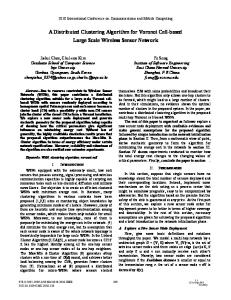
Chapter 6 – Results and analysis Experimental results where obtained on artificial data sets. As the performance is not dependant on the actual data distribution the synthetic data sets were composed of randomly placed data points. To observe the influence of the number of data points on the performance data sets with 500, 5000, 50.000 and 500.000 instances were created. For each instance count 3 data sets were created with 2, 20 and 200 dimensions. The sequential k-means implementation and the centroid update phase for the gpu-base k-means was coded in C using the Visual C++ 2008 compiler. For both compilers full optimizations were enabled, favoring speed over size as well as using processor specific extensions like SSE3. In the case of the Intel C++ compiler all vector related operations such as distance measurements, additions and scaling were vectorized using SSE3. The CUDA portions of the code were compiled using the CUDA Toolkit 2.0.

Fig 11 Speedup against instance count and dimensions 53

The test system was composed of an Intel Core 2 Duo E8400 CPU, 4 GB RAM running Windows XP Professional with Service Pack 3. The GPU was an NVIDIA GeForce 9600 GT hosting 512 MB of RAM, the driver used was the NVIDIA driver for Windows XP with CUDA support version 178.08.

Fig 12 Percentage of time used for various stages on GPU

The figures present the speedups gained by using the GPU for the labeling stage. While full optimizations were turned on for the Visual C++ the GPUbased implementation outperformed it by a factor of 4 to 43 for all but the smallest data set. A clear increase in performance can be observed the higher the number of instances dimensions and clusters. For the fully optimized Intel C++ version the speedups are obviously smaller as this version makes use of the SIMD instruction-set of the CPU. A speedup by a factor of 1.5 to 14 can be observed for all but the smallest data set. Interestingly this version performs better for lower dimensionality for high instance counts. This is due to the fact that as the centroid update 54

time decreases due to optimization the transfer time starts to play a bigger role. Nevertheless there is still a considerable speedup observable. The diagrams also explain why the GPU based implementation does not match the CPU implementation for very small data sets. From the plot it can be seen that for 500 data points nearly all the time is spent on the GPU. This time span also includes the calling overhead for invoking the GPU labeling stage. This invocation time actually takes longer than labeling the data items. The GPU-based implementation is clearly memory bound as there are more memory accesses than floating point operations. Therefore the approximate data throughput rate for the labeling stage was also computed. The values ranged from 23GB/s to 44GB/s depending on the instance and cluster count as well as dimensionality. For the used hardware the peak performance is given as 57.6 GB/s. Therefore we are highly confident that the implementation is nearly optimal. Due to being memory bound the GFLOP counts do of course not reach the hardwares peak values. 26GFLOP/s to 36GFLOP/s could be achieved approximately. For some test runs slight variations in the resulting centroids were observed. These variations are due to the use of combined multiplication and addition operations (MADD) that introduce rounding errors. Quantifying these errors was out of the scope of this work, especially as no information from the vendor on the matter was available.

55

Chapter 7 – Conclusion and future expansion Exploiting the GPU for the labeling stage of k-means proved to be beneficial especially for large data sets and high cluster counts. The presented implementation is only limited in the available memory on the GPU and therefore scales well. However, some drawbacks are still present. Many real-life data sets like document collections operate in very high dimensional spaces where document vectors are sparse. The implementation of linear algebra operations on sparse data on the GPU has yet to be solved optimally. Necessary access patterns such as memory coalescing make this a very hard undertaking. Also, the implementation presented is memory bound meaning that not all of the GPUs computational power is harvested. Finally, due to rounding errors the results might not equal the results obtained by a pure CPU implementation. However, our experimental experience showed that the error is negligible. Future work will involve experimenting with other k-means variations such as spherical or kernel k-means that promise to increase the computational load and therefore better suit the GPU paradigm. Also, an efficient implementation of the centroid update stage on the GPU will be investigated. This work compared the performance of CPU and GPU implementations of three, naturally data-parallel applications: traffic simulation, thermal simulation, and k-means. Our experiments used NVIDIA’s C-based CUDA interface and compared performance on an NVIDIA Geforce 8800 GTX with that on an Intel Pentium 4 CPU. Even though we did not perform extensive performance tuning, the GPU implementations of these applications obtained impressive speedups and add to the growing body of GPGPU work showing the potential of GPUs for general-purpose computing. Furthermore, the CUDA interface made programming these applications vastly easier than traditional rendering based GPGPU approaches (in particular, we have prior experience with structured grids). We also believe that the availability of shared memory and the domain abstraction provided by CUDA made these applications vastly easier to implement than traditional SPMD/thread-based approaches. 56

In the case of k-means and the traffic simulation, CUDA was probably a bit more difficult than OpenMP, chiefly due to the need to explicitly move data and deal with the GPU’s heterogeneous memory model. In the case of HotSpot with the pyramidal implementation, CUDA’s “grid-of-blocks” paradigm probably simplified implementation compared to OpenMP. The work we presented in this research thesis only shows a developmental stage of our work. We plan to extend our GPGPU work by comparing with more recent commodity configurations such as Intel dual-core processors and examining the programmability of more complex applications with various kinds of data structures and memory access patterns. In addition, in order to better understand the pros and cons of GPU architectures for general-purpose parallel programming, new metrics are needed for characterizing the applications. With greater architectural convergence of CPUs and GPUs, our goal is to find a parallel programming model that can best aid developers to program in today’s high-performance parallel computing environments, including GPUs and multi-core CPUs.

57

References •

Jian Yi, Yuxin Peng, and Jianguo Xiao. Color-based clustering for text detection and extraction in image. In MULTIMEDIA ’07: Proceedings of the 15th international conference on Multimedia, pages 847–850, New York, NY, USA, 2007. ACM.

•

Dannie Durand and David Sankoff. Tests for gene clustering. In RECOMB ’02: Proceedings of the sixth annual international conference on Computational biology, pages 144–154, New York, NY, USA, 2002.

•

Adil M. Bagirov and Karim Mardaneh. Modified global k-means algorithm for clustering in gene expression data sets. In WISB ’06: Proceedings of the 2006 workshop on Intelligent systems for bioinformatics, pages 23–28, Darlinghurst, Australia, Australia, 2006. Australian Computer Society, Inc.

•

Shi Zhong. Efficient streaming text clustering. Neural Netw., 18(5-6):790–798, 2005.

•

Stuart P. Lloyd. Least squares quantization in pcm. IEEE Transactions on Information Theory, 28(2):129–136, 1982.

•

J. B. MacQueen. Some methods for classification and analysis of multivariate observations. In L. M. Le Cam and J. Neyman, editors, Proc. of the fifth Berkeley Symposium on Mathematical Statistics and Probability, volume 1, pages 281–297. University of California Press, 1967.

•

David Arthur and Sergei Vassilvitskii. k-means++: the advantages of careful seeding. In Nikhil Bansal, Kirk Pruhs, and Clifford Stein, editors, SODA, pages 1027–1035. SIAM, 2007.

•

Jens Kr¨ uger and R¨ udiger Westermann. Linear algebra operators for gpu implementation of numerical algorithms. In SIGGRAPH ’03: ACM SIGGRAPH 2003 Papers, pages 908–916, New York, NY, USA, 2003. ACM.

•

Ian Buck, Tim Foley, Daniel Horn, Jeremy Sugerman, Kayvon Fatahalian, Mike Houston, and Pat Hanrahan. Brook for gpus: stream computing on graphics hardware. In SIGGRAPH ’04: ACM SIGGRAPH 2004Papers, pages 777–786, New York, NY, USA, 2004.

•

Mark Harris. Mapping computational concepts to gpus. In SIGGRAPH ’05: ACM SIGGRAPH 2005 Courses, page 50, New York, NY, USA, 2005. ACM.

•

Nvidia cuda site, 2010. 58

•

Hiroyuki Takizawa and Hiroaki Kobayashi. Hierarchical parallel processing of large scale data clustering on a pc cluster with gpu coprocessing. J. Supercomput., 36(3):219–234, 2006.

•

Jesse D. Hall and John C. Hart. Gpu acceleration of iterative clustering. Manuscript accompanying poster at GP2: The ACM Workshop on General Purpose Computing on Graphics Processors, and SIGGRAPH 2004.

•

Leon Bottou and Yoshua Bengio. Convergence properties of the K-means algorithms. In G. Tesauro, D. Touretzky, and T. Leen, editors, Advances in Neural Information Processing Systems, volume 7, pages585–592. The MIT Press, 1995.

59

Appendix kmean.cu // includes, system #include #include #include #include // includes, project #include // includes, kernels #include // declaration, forward void swap(void **a, void **b) { void * temp= *a; *a = *b; *b = temp; } __host__ void getInput(int *n, int *m, int *k, float *threshold, float **h_dataptx, float **h_datapty); __host__ void runTest( int n, int m, int k, float threshold, float *h_dataptx, float *h_datapty); extern "C" void computeGold( const int& n, const int& m, const int& k, const float& threshold, const float *const x, const float *const y, float *const ref_centriodx, float *const ref_centriody, int *const ref_clusterno, int *const ref_numIter); //////////////////////////////////////////////////////////////////////////////// // Program main //////////////////////////////////////////////////////////////////////////////// int main( int argc, char** argv) { int n,m,k; float *h_dataptx,*h_datapty; float threshold; getInput( &n, &m, &k, &threshold, &h_dataptx, &h_datapty); CUT_DEVICE_INIT(argc, argv); runTest(n, m, k, threshold, h_dataptx, h_datapty); free(h_dataptx); free(h_datapty); 60

CUT_EXIT(argc, argv); } __host__ void getInput(int *n, int *m, int *k, float *threshold, float **h_dataptx, float **h_datapty) { FILE* fin = fopen( "n200000k50.in", "r"); fscanf(fin, "%d%d", n, k); fscanf(fin, "%d%f", m, threshold); *h_dataptx = (float*) malloc(sizeof(float)*(*n)); *h_datapty = (float*) malloc(sizeof(float)*(*n)); for ( int i = 0; i < *n; ++i) fscanf(fin, "%f%f", *h_dataptx+i, *h_datapty+i); } //////////////////////////////////////////////////////////////////////////////// //! Run a simple test for CUDA //////////////////////////////////////////////////////////////////////////////// __host__ void runTest( int n, int m, int k, float threshold, float *h_dataptx, float *h_datapty) { //CUT_DEVICE_INIT(); unsigned int timer = 0; CUT_SAFE_CALL( cutCreateTimer( &timer)); CUT_SAFE_CALL( cutStartTimer( timer)); const int num_blocks = 1 + ( (n-1) >> LOG_BLOCKDIM ); const unsigned int mem_length = (((num_blocks-1)>>LOG_HALF_WARP) + 1) << LOG_HALF_WARP; // allocate device memory float *d_dataptx, *d_datapty; CUDA_SAFE_CALL( cudaMalloc( (void**) &d_dataptx, sizeof(float)*n)); CUDA_SAFE_CALL( cudaMalloc( (void**) &d_datapty, sizeof(float)*n)); float *d_centriodx, *d_centriody; CUDA_SAFE_CALL( cudaMalloc( (void**) &d_centriodx, sizeof(float)*k )); CUDA_SAFE_CALL( cudaMalloc( (void**) &d_centriody, sizeof(float)*k )); // copy host memory to device CUDA_SAFE_CALL( cudaMemcpy( d_dataptx, h_dataptx, sizeof(float)*n, cudaMemcpyHostToDevice) ); CUDA_SAFE_CALL( cudaMemcpy( d_datapty, h_datapty, sizeof(float)*n, cudaMemcpyHostToDevice) ); cudaThreadSynchronize(); CUDA_SAFE_CALL( cudaMemcpy( d_centriodx, d_dataptx, sizeof(float)*k, cudaMemcpyDeviceToDevice) ); CUDA_SAFE_CALL( cudaMemcpy( d_centriody, d_datapty, sizeof(float)*k, cudaMemcpyDeviceToDevice) ); // allocate device memory for result 61

float *d_sumx[2], *d_sumy[2]; int *d_count[2]; for(int i = 0; i < 2; ++i) { CUDA_SAFE_CALL( cudaMalloc( (void**) &d_sumx[i], sizeof(float)*mem_length*k )); CUDA_SAFE_CALL( cudaMalloc( (void**) &d_sumy[i], sizeof(float)*mem_length*k )); CUDA_SAFE_CALL( cudaMalloc( (void**) &d_count[i], sizeof(int)*mem_length*k )); } int *d_clusterno; CUDA_SAFE_CALL( cudaMalloc( (void**) &d_clusterno, sizeof(int)*n )); bool *d_flag; CUDA_SAFE_CALL( cudaMalloc( (void**) &d_flag, sizeof(bool))); cudaThreadSynchronize(); bool flag=true; int numIter; for( numIter = 0; flag && numIter < m; ++numIter ) { cluster <<< dim3(num_blocks), dim3(BLOCKDIM), k*(sizeof(float)<<1) >>> (n, k, d_dataptx, d_datapty, d_centriodx, d_centriody, d_sumx[0], d_sumy[0], d_count[0]); cudaThreadSynchronize(); for (int len = num_blocks; len != 1; len = 1+((len-1)>>(LOG_BLOCKDIM+1))) { summation <<< dim3(1+((len-1)>>(LOG_BLOCKDIM+1))) , dim3(BLOCKDIM) >>> (n, k, len, d_sumx[0], d_sumy[0], d_count[0], d_sumx[1], d_sumy[1], d_count[1]); cudaThreadSynchronize(); swap((void**)&d_sumx[0],(void**)&d_sumx[1]); swap((void**)&d_sumy[0],(void**)&d_sumy[1]); swap((void**)&d_count[0],(void**)&d_count[1]); } flag = false; CUDA_SAFE_CALL( cudaMemcpy( d_flag, &flag, sizeof(bool), cudaMemcpyHostToDevice) ); cudaThreadSynchronize(); computeCentriod <<< dim3(1+((k-1)>>LOG_BLOCKDIM)) , dim3(BLOCKDIM) >>> (n, k, threshold,d_centriodx,d_centriody,d_sumx[0],d_sumy[0],d_count[0], d_flag); cudaThreadSynchronize(); CUDA_SAFE_CALL( cudaMemcpy( &flag, d_flag, sizeof(bool), cudaMemcpyDeviceToHost) ); cudaThreadSynchronize(); }

62

findCluster <<< dim3(num_blocks), dim3(BLOCKDIM), k*(sizeof(float)<<1) >>> (n, k, d_dataptx, d_datapty, d_centriodx, d_centriody, d_clusterno); cudaThreadSynchronize(); // check if kernel execution generated and error CUT_CHECK_ERROR("Kernel execution failed"); float *h_centriodx = (float*) malloc(sizeof(float)*k); float *h_centriody = (float*) malloc(sizeof(float)*k); CUDA_SAFE_CALL( cudaMemcpy( h_centriodx, d_centriodx, sizeof(float)*k, cudaMemcpyDeviceToHost) ); CUDA_SAFE_CALL( cudaMemcpy( h_centriody, d_centriody, sizeof(float)*k, cudaMemcpyDeviceToHost) ); int *h_clusterno = (int*) malloc(sizeof(int)*n); CUDA_SAFE_CALL( cudaMemcpy( h_clusterno, d_clusterno, sizeof(int)*n, cudaMemcpyDeviceToHost) ); CUDA_SAFE_CALL(cudaFree(d_dataptx)); CUDA_SAFE_CALL(cudaFree(d_datapty)); CUDA_SAFE_CALL(cudaFree(d_centriodx)); CUDA_SAFE_CALL(cudaFree(d_centriody)); for(int i = 0; i < 2; ++i) { CUDA_SAFE_CALL( cudaFree(d_sumx[i]) ); CUDA_SAFE_CALL( cudaFree(d_sumy[i]) ); CUDA_SAFE_CALL( cudaFree(d_count[i]) ); } CUT_SAFE_CALL( cutStopTimer( timer)); printf( "GPU version processing time: %f (ms)\n", cutGetTimerValue( timer)); CUT_SAFE_CALL( cutDeleteTimer( timer)); printf( "GPU version number of iterations: %d\n", numIter);

// compute reference solution timer = 0; CUT_SAFE_CALL( cutCreateTimer( &timer)); CUT_SAFE_CALL( cutStartTimer( timer)); float* ref_centriodx = (float*) malloc(sizeof(float)*k); float* ref_centriody = (float*) malloc(sizeof(float)*k); int* ref_clusterno = (int*) malloc(sizeof(int)*n); int ref_numIter; computeGold( n, m, k, threshold, h_dataptx, h_datapty, ref_centriodx, ref_centriody, ref_clusterno, &ref_numIter); CUT_SAFE_CALL( cutStopTimer( timer)); printf( "CPU version processing time: %f (ms)\n", cutGetTimerValue( timer)); 63

CUT_SAFE_CALL( cutDeleteTimer( timer)); printf( "CPU version number of iterations: %d\n", ref_numIter); /*bool b_numIter = (numIter == ref_numIter); bool b_x = (memcmp(h_centriodx, ref_centriodx, sizeof(float)*k)==0); bool b_y = (memcmp(h_centriody, ref_centriody, sizeof(float)*k)==0); bool b_c = (memcmp(h_clusterno, ref_clusterno, sizeof(int)*n)==0); printf( "numIter: Test %s\n", (b_numIter) ? "PASSED" : "FAILED"); printf( "b_x: Test %s\n", (b_x) ? "PASSED" : "FAILED"); printf( "b_y: Test %s\n", (b_y) ? "PASSED" : "FAILED"); printf( "b_c: Test %s\n", (b_c) ? "PASSED" : "FAILED"); for(int i=0;i!=k;++i) { if(h_centriodx[i]!=ref_centriodx[i]) printf("%f %f\n",h_centriodx[i],ref_centriodx[i]); if(h_centriody[i]!=ref_centriody[i]) printf("%f %f\n",h_centriody[i],ref_centriody[i]); }*/ // cleanup memory free( h_centriodx); free( h_centriody); free(h_clusterno); free(ref_centriodx); free(ref_centriody); free(ref_clusterno); }

64

kmean.cpp #include #include #include float distance(const float &x1, const float &y1, const float &x2, const float &y2) {return sqrtf((x2-x1)*(x2-x1)+(y2-y1)*(y2-y1));} //////////////////////////////////////////////////////////////////////////////// // export C interface extern "C" void computeGold( const int& n, const int& m, const int& k, const float& threshold, const float *const x, const float *const y, float *const ref_centriodx, float *const ref_centriody, int *const ref_clusterno, int *const ref_numIter); void computeGold( const int& n, const int& m, const int& k, const float& threshold, const float *const x, const float *const y, float *const ref_centriodx, float *const ref_centriody, int *const ref_clusterno, int *const ref_numIter) { int* count = (int*) malloc(sizeof(int)*k); float* prev_centriodx = (float*) malloc(sizeof(float)*k); float* prev_centriody = (float*) malloc(sizeof(float)*k); for(int i=0;i!=n;++i) ref_clusterno[i]=i; int flag=true; for(*ref_numIter = -1; flag && *ref_numIter < m; ++ *ref_numIter) { flag=(*ref_numIter<0); //compute centriod for(int j=0;j!=k;++j) { count[j]=0; prev_centriodx[j] = (*ref_numIter == 0)? x[j] : ref_centriodx[j]; prev_centriody[j] = (*ref_numIter == 0)? y[j] : ref_centriody[j]; ref_centriodx[j]=ref_centriody[j]=0; } for(int i=0;i!=n;++i) if(ref_clusterno[i]
ref_centriodx[j]/=count[j]; ref_centriody[j]/=count[j]; if(distance(ref_centriodx[j],ref_centriody[j],prev_centriodx[j],prev_centriody[j]) >= threshold * n) { //printf("Bingo!\n"); flag = true; } } //cluster for(int i=0;i!=n;++i) { int temp=0; for(int j=0;j!=k;++j) if(distance(x[i],y[i],ref_centriodx[j],ref_centriody[j])
66

kmean_kernel.cu #ifndef _TEMPLATE_KERNEL_H_ #define _TEMPLATE_KERNEL_H_ #define LOG_HALF_WARP 4 #define LOG_NUM_BANKS 4 #define LOG_BLOCKDIM 8 #define BLOCKDIM (1<> LOG_NUM_BANKS)) #include __device__ float distance(const float &x1, const float &y1, const float &x2, const float &y2) {return sqrtf((x2-x1)*(x2-x1)+(y2-y1)*(y2-y1));} __global__ void cluster(int n, int k, const float *const d_dataptx, const float *const d_datapty, float *d_centriodx, float *d_centriody, float *d_sumx, float *d_sumy, int *d_count) { // shared memory extern __shared__ float s_centriod[]; __shared__ float s_sumx[BLOCKDIM<<1]; __shared__ float s_sumy[BLOCKDIM<<1]; __shared__ float s_count[BLOCKDIM<<1]; const unsigned int index = (blockIdx.x << LOG_BLOCKDIM) + threadIdx.x; int closestNum; const unsigned int mem_length = (( (n-1) >> (LOG_BLOCKDIM + LOG_HALF_WARP)) + 1) << LOG_HALF_WARP; float *const s_centriodx = s_centriod; float *const s_centriody = s_centriod+k; float ptx,pty; //coalesced access __syncthreads(); for(int i = 0; i < k; i+=BLOCKDIM) if( i + threadIdx.x < k) { s_centriodx[i+threadIdx.x] = d_centriodx[i+threadIdx.x]; s_centriody[i+threadIdx.x] = d_centriody[i+threadIdx.x]; } __syncthreads(); if(index
pty = d_datapty[index]; closestNum = 0; for(int i = 1; i < k; ++i) { if( distance( ptx, pty, s_centriodx[i], s_centriody[i]) < distance( ptx, pty, s_centriodx[closestNum], s_centriody[closestNum]) ) { closestNum = i; } } } for(int i = 0; i < k; ++ i) { __syncthreads(); if(index
} __global__ void summation(int n,int k,int len, float *d_sumx, float *d_sumy, int *d_count, float *d_sumx_aux, float *d_sumy_aux, int *d_count_aux) { //shared __shared__ float s_sumx[BLOCKDIM<<2]; __shared__ float s_sumy[BLOCKDIM<<2]; __shared__ int s_count[BLOCKDIM<<2]; const unsigned int mem_length = (( (n-1) >> (LOG_BLOCKDIM + LOG_HALF_WARP)) + 1) << LOG_HALF_WARP; for(int i = 0; i < k; ++i) { unsigned int index = i * mem_length + (blockIdx.x<<(LOG_BLOCKDIM+1)) + threadIdx.x; __syncthreads(); if((blockIdx.x<<(LOG_BLOCKDIM+1)) + threadIdx.x
{ __syncthreads(); if(threadIdx.x < 1<<(LOG_BLOCKDIM-depth) ) { s_count[CONFLICT_FREE_INDEX( threadIdx.x<<(depth+1) )] += s_count[CONFLICT_FREE_INDEX( (threadIdx.x<<(depth+1)) + (1<> (LOG_BLOCKDIM + LOG_HALF_WARP)) + 1) << LOG_HALF_WARP; const unsigned int index = (blockIdx.x << LOG_BLOCKDIM) + threadIdx.x; float sumx, sumy, centriodx,centriody; int count; __syncthreads(); if(index
//printf("%d %f %d\n",threadIdx.x,d_sumx[threadIdx.x],d_count[threadIdx.x*mem_length]); } else { s_flag[CONFLICT_FREE_INDEX( threadIdx.x )] = 0.0f; } __syncthreads(); if(threadIdx.x0) { *d_flag=true; } } __global__ void findCluster( int n, int k, const float *const d_dataptx, const float *const d_datapty, float *d_centriodx, float *d_centriody, int *d_clusterno ) { // shared memory extern __shared__ float s_centriod[]; unsigned int index = (blockIdx.x << LOG_BLOCKDIM) + threadIdx.x; int closestNum; float *const s_centriodx = s_centriod; float *const s_centriody = s_centriod+k; float ptx,pty; __syncthreads(); for(int i = 0; i < k; i+=BLOCKDIM) if( i + threadIdx.x < k) { s_centriodx[i+threadIdx.x] = d_centriodx[i+threadIdx.x]; s_centriody[i+threadIdx.x] = d_centriody[i+threadIdx.x]; 71

} __syncthreads(); if(index
72