TACO, 3(2):115-155, 2006.
A Lifetime Optimal Algorithm for Speculative PRE Jingling Xue and Qiong Cai University of New South Wales
A lifetime optimal algorithm, called MC-PRE, is presented for the first time that performs speculative PRE based on edge profiles. In addition to being computationally optimal in the sense that the total number of dynamic computations for an expression in the transformed code is minimized, MC-PRE is also lifetime optimal since the lifetimes of introduced temporaries are also minimized. The key in achieving lifetime optimality lies not only in finding a unique minimum cut on a transformed graph of a given CFG but also in performing a data-flow analysis directly on the CFG to avoid making unnecessary code insertions and deletions. The lifetime optimal results are rigorously proved. We evaluate our algorithm in GCC against three previously published PRE algorithms, namely, MC-PREcomp (Qiong and Xue’s computationally optimal version of MC-PRE), LCM (Knoop, R¨ uthing and Steffen’s lifetime optimal algorithm for performing non-speculative PRE) and CMP-PRE (Bodik, Gupta and Soffa’s PRE algorithm based on code-motion preventing (CMP) regions, which is speculative but not computationally optimal). We report and analyze our experimental results, obtained from both actual program execution and instrumentation, for all 22 C, C++ and FORTRAN 77 benchmarks from SPECcpu2000 on an Itanium 2 computer system. Our results show that MC-PRE (or MC-PREcomp ) is capable of eliminating more partial redundancies than both LCM and CMP-PRE (especially in functions with complex control flow), and in addition, MC-PRE inserts temporaries with shorter lifetimes than MC-PREcomp . Each of both benefits has contributed to the performance improvements in benchmark programs at the costs of only small compile-time and code-size increases in some benchmarks. Categories and Subject Descriptors: D.3.4 [Programming Languages]: Processors—compilers; optimization; F.2.2 [Analysis of Algorithms and Problem Complexity]: Non-numerical algorithms and problems; G.2.2 [Discrete Mathematics]: Graph Theory—Graph algorithms; network problems General Terms: Algorithms, Languages, Experimentation, Performance Additional Key Words and Phrases: Partial redundancy elimination, classic PRE, speculative PRE, computational optimality, lifetime optimality, data flow analysis
1. INTRODUCTION Partial redundancy elimination (PRE) is a powerful and widely used optimization technique aimed at removing computations that are redundant due to recomputing previously computed values [Morel and Renvoise 1979]. PRE is attractive because by targeting computations that are redundant only along some paths in a CFG, it encompasses global common subexpression elimination (GCSE), loopinvariant code motion (LICM), and more. As a result, PRE is an important component in global optimizers. Traditionally, PRE has been implemented as a profile-independent optimization. For example, GCC 3.4.3 consists of a pass for performing PRE, which is based on the well-known algorithm called lazy code moAuthors’ address: Programming Languages and Compilers Group, School of Computer Science and Engineering, University of New South Wales, Sydney, NSW 2052, Australia.
tion (LCM) [Knoop et al. 1994]. As another example, Open64 conducts PRE in static single assignment (SSA) form [Cytron et al. 1991]) using the SSAPRE algorithm described in [Kennedy et al. 1999]. These classic PRE algorithms guarantee both computationally and lifetime optimal results: the number of computations cannot be reduced any further by safe code motion [Kennedy 1972] and the lifetimes of introduced temporaries are minimized. Under such a safety constraint, they remove partial redundancies along some paths but never introduce additional computations along any path that did not contain them originally. In real programs, some points (nodes or edges) in a CFG are executed more frequently than others. If we have their execution frequencies available and if we know that an expression cannot cause an exception, we can perform code motion transformations missed by the classic PRE algorithms. The central idea is to use control speculation (i.e., unconditional execution of an expression that is otherwise executed conditionally) to enable the removal of partial redundancies along some more frequently executed paths at the expense of introducing additional computations along some less frequently executed paths. Such a speculative PRE may potentially insert computations on paths that did not execute them in the original program. As a result, the safety criterion enforced in classic PRE is relaxed. There are three computationally optimal algorithms for solving the speculative PRE problem [Bodik 1999; Cai and Xue 2003; Scholz et al. 2004]. However, none of them is also lifetime optimal. Bodik et al. [1998] have also introduced a speculative PRE algorithm, which is referred to as CMP-PRE in this paper, based on codemotion-preventing (CMP) regions. They show that CMP-PRE can eliminate more partially redundant computations than LCM despite its being non-computationally optimal. This paper presents the first algorithm that achieves both computational and lifetime optimal results simultaneously. Presently, many existing compiler frameworks have incorporated and used profiling information to support control speculation (and data speculation [Lin et al. 2003]). As increasingly more aggressive profile-guided optimizations are being employed, the profiling overhead can be better amortized (or shared). However, profile-guided speculative PRE algorithms are yet to be incorporated into existing compiler frameworks. As mentioned above, GCC supports LCM (which is non-speculative) while Open64 embraces SSAPRE (which, combined with the extension described in [Lo et al. 1998], can promote register reuse by performing speculative loads and stores). In summary, this paper makes the following contributions: Lifetime Optimality. We present the first lifetime optimal algorithm, MC-PRE (the “MC” stands for Min-Cut), for performing speculative PRE from edge profiles. In addition to being computationally optimal, MC-PRE is also lifetime optimal. The key in achieving the lifetime optimality lies not only in finding a unique minimum cut on a transformed graph of a given CFG but also in performing a data-flow analysis on the CFG to avoid making unnecessary code insertions and replacements for isolated computations. The lifetime optimal results are rigorously proved. Algorithm. Our computationally optimal algorithm described in [Cai and Xue 2003] assumes single statement blocks. This paper presents our lifetime optimal algorithm in terms of standard basic blocks so that it is directly implementable. Implementations. We have implemented MC-PRE in GCC (GNU Compiler Collection) 3.4.3. We make use of the bit-vector routines in GCC to perform our data2
flow analysis passes. This is also the same framework used by the LCM algorithm implemented in GCC. In performing the min-cut part of our algorithm, we use Goldberg’s push-relabel HIPR algorithm [Goldberg 2003] and his implementation, which is one of the fastest implementations available [Chekuri et al. 1997]. As a result, we have also obtained an implementation of our earlier PRE algorithm [Cai and Xue 2003] in GCC. This precursor of MC-PRE, denoted MC-PREcomp , is computationally optimal but not lifetime optimal. For comparison purposes, we have also implemented Bodik, Gupta and Soffa’s CMP-PRE algorithm [Bodik et al. 1998], which uses a non-Boolean lattice with three values. The data-flow analyses required by CMP-PRE are carried out using modified versions of GCC’s bit-vector routines. Eliminated Computations. We evaluate MC-PRE against LCM and CMP-PRE using all 22 SPECcpu2000 benchmarks on Itanium 2 in terms of redundant computations eliminated. MC-PRE eliminates more non-full (i.e., strictly partial) redundancies than LCM and more non-full redundancies that are only speculatively removable (i.e., that are not removable by LCM) than CMP-PRE. This is particularly pronounced for functions with complex control flow. In the case of SPECint2000, MC-PRE removes between 31.39% and 147.56% (an average of 90.13%) more non-full redundancies than LCM and between 0.52% and 280.47% (an average of 58.15%) more non-full redundancies that are only speculatively removable than CMP-PRE. In the case of SPECfp2000, these percentage increases are 0.10% – 264.67% (33.84%) over LCM and 0.00% – 89.98% (15.23%) over CMP-PRE. Lifetimes of Introduced Temporaries. MC-PRE uses insertions with shorter lifetimes than MC-PREcomp in all 22 benchmarks used. In addition, MC-PRE is comparable with or better than LCM and CMP-PRE in terms of this criterion in these benchmarks despite that these two previous PRE algorithms are not computationally optimal for solving the speculative PRE problem. Performance Improvements. By eliminating more redundant computations than LCM and CMP-PRE and using insertions with the shortest lifetimes possible (shorter than MC-PREcomp ), MC-PRE achieves nearly the same or better performance results than the other three PRE algorithms in all 22 benchmarks. By keeping the lifetimes of introduced temporaries to a minimum, MC-PRE yields faster codes than MC-PREcomp in 19 of these benchmarks. In the case of SPECint2000, MC-PRE outperforms MC-PREcomp , LCM and CMP-PRE in nearly all its 12 benchmarks. In the case of SPECfp2000, LCM has succeeded in eliminating over 80% of the non-full redundancies in nine out of its 10 benchmarks. However, MC-PRE still achieves nearly the same or better performance results in these benchmarks than the other three algorithms. MC-PRE is optimal since it can eliminate all partial (full and non-full) redundancies by using temporaries with the shortest lifetimes possible as long as they can be eliminated profitably (with respect to a given edge profile). As a result, MC-PRE can potentially achieve better performance than LCM and CMP-PRE even in programs where LCM and CMP-PRE have eliminated most of their non-full redundancies. This has happened to mesa and sixtrack in the SPECfp2000 suite. For sixtrack, MC-PRE achieves a speedup of 7.03% over LCM since all non-full redundancies that MC-PRE eliminates but LCM does not are from its hottest functions. For mesa, MC-PRE achieves a speedup of 5.75% (5.73%) over LCM (CMP-PRE) since MC-PRE has eliminated redundant computations from a number of expensive expressions that both LCM and CMP-PRE 3
have failed to remove in one of its hottest functions. Low Compilation Overhead. Conventional wisdom suggests that a min-cut solver may be too expensive to be practically useful in our setting. Instead of directly operating on CFGs, a min-cut solver operates on significantly reduced subgraphs of CFGs. As a result, MC-PRE incurs only small extra compilation overheads relative to LCM. By replacing LCM with MC-PRE, GCC has only moderate increases in compile times across 22 SPECcpu2000 benchmark programs. The compile times from MC-PRE, MC-PREcomp and CMP-PRE do not differ significantly. Low Space Overhead. A PRE algorithm inserts and deletes computations in a program. As a result, it may cause the static code size in a program to be increased or decreased. MC-PRE are comparable with LCM and CMP-PRE in terms of this criterion while MC-PREcomp results in slightly larger binaries in some benchmarks. PRE is almost universally used in optimizing compilers. The experimental results as summarized above show that MC-PRE can be practically employed as a PRE pass in a profile-guided optimizing compiler framework. We illustrate the basic idea of our algorithm using an example given in Figure 1 by focussing on one single PRE candidate expression, a + b. After the local PRE pass has been performed within basic blocks, there are only two kinds of candidate computations of a + b to be dealt with by the global PRE pass: UB = {2, 4, 10, 11, 13} DB = {6, 11}
(1)
where UB is the set of blocks where a + b is upwards exposed and DB is the set of blocks where a + b is both downwards exposed and preceded by assignments to a or b. (Note that UB and DB are not symmetrically defined in this paper.) MC-PRE starts with by performing two standard data-flow analyses — the forward availability and the backward partial anticipatability — on the CFG given in Figure 1(a) to identify all non-essential edges and nodes. Figure 1(b) duplicates the CFG given in Figure 1(a) with all the non-essential edges and nodes being depicted in dashes. By removing these non-essential edges and nodes from the given CFG, we obtain the reduced graph as shown in Figure 1(c). This reduced graph is then transformed into the so-called essential flow graph (EFG), which is an s-t flow network given in Figure 1(d). We apply a min-cut algorithm to the EFG to obtain the minimum cut as illustrated in Figure 1(d). Let C1 denote this minimum cut: C1 = {(1, 2), (3, 4), (5, 7)} At this stage, the following transformation, CO 1 , is computationally optimal: U-INSCO1 = C1 = {(1, 2), (3, 4), (5, 7)} U-DELCO1 = UB = {2, 4, 10, 11, 13} D-INSDELCO1 = DB = {6, 11}
(2)
This transformation would be lifetime optimal if insertions and deletions for isolated computations were allowed. Thus, such an almost-lifetime optimal transformation corresponds to the Almost LCM transformation in classic PRE [Knoop et al. 1992; 1994]. For illustration purposes, Figure 1(e) depicts the transformed code, which is not actually generated. The first two sets prescribe the insertions and replacements 4
� ��� � ! ���� �� � ����� " ����� # �� �� � �����
9 ����� �����
'
����� ���� �� � � � ���� ��� �
�� �� �
�����
(
�����
+� ! �����
% �����
�����
�� ��� ��# �
=
�����
$ �� ��� � ���
&
�� ��� *� " ���� �� � �����
> 3 .�2�04-
������� � ���� �� �
? 2�. 6;: -
B
C
9+<
9*= /�.�2�04-
�*) �� �� � �����
/�.�2�04- . 3�576 9�9 � 3 .�2�04-
U M�G�H�JPK V
Y
l
∞
~+
~] ~+
∞
∞
p o
I��
w �s vT| t�s�{�| w v�sut
u� ¡ �� �
��� ���
~]
r�sut �u � �y� I��
v�s t
}
(e) Almost-lifetime optimal solution Fig. 1.
_�n `aa
{�s�z� w t�s�{�| w
b+a a
���
v�s t
m
(d) Essential flow graph (EFG)
q
rIsut
b+a�a
d�a a
_]h
Q]V M�G�H�JPK
ts�{�| w
v�sut ~�~ w �s ryx�w z t�s�{�| rIsut
c a�a
^ o
c�a
__
(c) Reduced graph
k ∞
Q]\ F�GIH�JLK
∞
efa a
∞
j ∞
ts�{�| w
^
h
X H�G�OTS K
~
_
e a�a i
W FRG�H�JPK
M�GIH�JLK �Q Q K�G�F�N�O F�GIH�JLK
9+D 3 .�2�0 -
8
9�> efa a
g
[
-�.�/�0 1 /�.�2�0 -
(b) Availability and anticipatability analyses
E
Z
@
A
�����
(a) Original flow graph
Q
,
< /�.�2�04-
*
] �
* �
(f) Lifetime optimal solution
A running example illustrating our optimal algorithm.
5
Iu
for the upwards exposed computations in UB, respectively. The last set specifies the insertions and replacements for the downwards exposed computations in DB . This work recognizes that finding a special minimum cut alone is not sufficient to guarantee lifetime optimality for speculative PRE. In the transformed program shown in Figure 1(e), there are three isolated computations. The upwards exposed computation a + b in block 2 is isolated since the definition h = a + b inserted on the edge (1, 2) is used only in block 2 and becomes dead at its exit. The upwards exposed computation a + b in block 4 is also isolated similarly. The downwards exposed computation a + b in block 11 is isolated because the definition h = a + b inserted inside the block is dead at its exit. To avoid making these unnecessary insertions and associated deletions, MC-PRE performs a third data-flow analysis pass on the original CFG given in Figure 1(a). As a result, the unique lifetime optimal transformation, LO, found by MC-PRE is: U-INSLO = {(5, 7)} U-DELLO = {10, 11, 13} D-INSDELLO = {6}
(3)
Performing this code motion on the CFG in Figure 1(a) leads to the optimally transformed code shown in Figure 1(f). The dynamic number of computations for a + b has been reduced optimally from 2850 to 1900. (For the same expression, the reduction by the profile-independent LCM would be from 2850 to 2450.) The rest of this paper is organized as follows. Section 2 reviews the related work. Section 3 gives some background information and introduces the notions of computational optimality and lifetime optimality for speculative PRE. Section 4 presents the MC-PRE algorithm in a style that can be directly and efficiently implemented in a compiler, while stating some lemmas with proofs. In Section 5, we discuss some theoretical aspects of the algorithm and prove rigorously its correctness and optimality. In Section 6, we evaluate MC-PRE against MC-PREcomp , LCM and CMP-PRE using SPECcpu2000 on an Itanium 2 computer system. Section 7 concludes the paper and discusses some future work. 2. RELATED WORK PRE originated from the seminal work of Morel and Renvoise [Morel and Renvoise 1979] and was soon realized as an important optimization technique that subsumes GCSE and LICM. Morel and Renvoise’s data-flow framework is imperfect: it is bidirectional, provides no assurance for lifetime optimality and is profile-independent. In the past two decades, their work has undergone a number of refinements and extensions [Briggs and Cooper 1994; Chow 1983; Click 1995; Dhamdhere 1991; Dhamdhere et al. 1992; Drechsler and Stadel 1993; Hosking et al. 2001; Kennedy et al. 1999; Knoop 1998; Knoop et al. 1992; 1994; Rosen et al. 1988; R¨ uthing et al. 2000; Simpson 1996]. In particular, Knoop et al. [1994] describe a uni-directional bit-vector formulation, known as LCM, that is optimal by the criteria of computational optimality and lifetime optimality, and more recently, Kennedy et al. [1999] present an SSA-based framework that shares the same two optimality properties. In addition, Knoop et al. [2000] extend the LCM algorithm to handle predicated code. Hailperin [1998] generalizes LCM so that the generalized version also performs constant propagation and strength reduction. Kennedy et al. [1998] extend 6
the SSAPRE algorithm to perform strength reduction and linear function test replacement. Steffen et al. [1990] present a PRE algorithm achieving computational optimality with respect to the Herbrand interpretation and later [1991] a less powerful but more efficient variant together with an extension to uniformly cover also strength reduction. By combining global reassociation and global value numbering [Alpern et al. 1988], Briggs and Cooper [1994] can also eliminate redundancies for certain semantically-identical expressions. However, these previous research efforts are restricted by the safety code motion criterion [Kennedy 1972] and insensitive to the execution frequencies of a program point in a given CFG. Horspool and Ho [1997] and Gupta et al. [1998] introduce the first two algorithms on performing profile-guided speculative PRE. Due to the local heuristics used, both algorithms are not computationally optimal. Later, computationally optimal results are achieved by the three different algorithms described in [Bodik 1999; Cai and Xue 2003; Scholz et al. 2004], which all rely on finding a minimum cut to obtain the required insertion points. However, none of these three algorithms is also lifetime optimal due to the arbitrary minimum cuts chosen in their algorithms. Bodik [1999] suggested to achieve lifetime optimal results by choosing cut edges as close as possible to the sinks of his flow network; but the details of this suggestion are missing. In order to reduce the lifetimes of introduced temporaries, Bodik [1999] used a non-optimal algorithm (presented earlier in [Bodik et al. 1998] and denoted CMP-PRE here) to perform speculative PRE based on code-motionpreventing (CMP) regions. They show that CMP-PRE can eliminate more non-full redundancies than LCM despite its being non-computationally optimal. In this paper, we extend our earlier algorithm [Cai and Xue 2003] so that the new algorithm, MC-PRE, can also achieve lifetime optimality for the first time. As a result, MC-PRE introduces temporary registers only when necessary, with the shortest lifetimes possible. The lifetime optimality is achieved by finding not only a special minimum cut and but also performing one additional data-flow analysis to avoid making insertions and replacements for isolated computations. Bodik et al. [1998] apply control flow restructuring as an alternative to speculation to enable code motion. They implemented their algorithm in the IMPACT compiler [Chang et al. 1991] and evaluated its effectiveness using SPEC95. They found that the number of redundancies that cannot be removed by speculation alone is negligible. In addition, such a negligible number of redundancies is eliminated at the cost of over 30% code explosion for most benchmarks. Steffen [1996] eliminates all partial redundancies in a program essentially by unrolling the program as far as necessary and then attempting to minimize the potentially exponential code-size explosion by collapsing nodes that are so-called bisimilar. In this paper, MC-PRE achieves a complete removal of all partial redundancies removable by using control speculation from edge profiles at negligible space overheads. Lo et al. [1998] extend the SSAPRE algorithm to handle control speculation and register promotion. Their algorithm performs no worse than if speculation is not used but is not optimal. Lin et al. [2003] incorporate alias profiling information to support data speculation in the SSAPRE framework. 7
3. PRELIMINARIES Section 3.1 recalls some concepts and results about directed graphs, flow networks and defines the notion of minimum cut used. In Section 3.2, we introduce control flow graphs (CFGs) and the local predicates used in our data-flow analysis. In Section 3.3, we formulate speculative PRE as a code motion transformation and define its correctness, computational optimality and lifetime optimality. 3.1 Directed Graphs and Flow Networks Let G = (N, E) be a directed graph with the node set N and the edge set E. The notation pred(G, n) represents the set of all immediate predecessors of a node n and succ(G, n) the set of all its immediate successors in G: pred(G, n) = {m | (m, n) ∈ E} succ(G, n) = {m | (n, m) ∈ E}
(4)
A node m is a predecessor of a node n if m is an immediate predecessor of n or if m is a predecessor of an immediate predecessor of n. A path of G is a finite sequence of nodes n1 , . . . , nk such that ni ∈ succ(ni−1 ), for all 1 < i 6 k, and the length of the path is k. In this case, we write hn1 , . . . , nk i and refer to the sequence as a path from n1 to nk (inclusive). Any subsequence of a path is referred to as a subpath. A directed graph G = (N, E) is a flow network if it has two distinguished nodes, a source s and a sink t, and a nonnegative capacity (or weight) c(n, m) > 0 for each edge (n, m) ∈ E. If (n, m) 6∈ E, it is customary to assume that c(n, m) = 0 [Cormen et al. 1990]. For convenience, every node is assumed to lie on some path from the source s to the sink t. Thus, a flow network is connected (from s to t). Let S and T = N − S be a partition of N such that s ∈ S and t ∈ T . We denote by (S, T ) the set of all (directed) edges with tail in S and head in T : (S, T ) = {(n, m) ∈ E | n ∈ S, m ∈ T }
(5)
A cut separating s from t is any edge set (C, C), where s ∈ C, C = N − C is the complement of C and t ∈ C. The capacity of this cut, denoted by cap(C, C), is the sum of the capacities of all the edges in the cut (called cut edges): X cap(C, C) = c(m, n) (6) (m,n)∈(C, C)
By a minimum cut, we mean a cut separating s from t with minimum capacity. 3.2 Control Flow Graphs A control flow graph (CFG) is a directed graph annotated with an edge profile. We represent a CFG as a weighted graph G = (N, E, W ), where N is the set of basic blocks, E the set of control flow edges, and W : E 7→ IN is the set of non-negative integers representing the execution frequencies of all flow edges. In addition, s ∈ N denotes the unique entry block without any predecessors and t ∈ N the unique exit block without any successors. Furthermore, every block is assumed to lie on some path from s to t. For convenience, we also write W (n) to represent the execution frequency of a block n ∈ N . Nodes and (basic) blocks are interchangeable. The profiling information input to a profile-guided algorithm provides only an approximation of actual execution frequencies. Therefore, an edge or node with a 8
�
�
�� ��� ��������� �����
����� ��������� ����� �
�
����� ����� ����� �����
Fig. 2. Profitability in partial redundancy elimination by using control speculation. Although being partially redundant, a+b in block 5 will not be eliminated since it is not profitably removable.
zero frequency is interpreted as least frequently rather than never executed at all. Assumption 3.1. For every node or edge x in G, its execution frequency is assumed to be nonzero, i.e., W (x) > 0. Assumption 3.2. The following assumption about an edge profile is made: X X W (n, m) W (n) = W (m, n) = m∈succ(G,n) m∈pred(G,n)
(7)
In all example CFGs used for illustrations, variables with distinct names are consistently meant to be distinct (i.e., not aliased to each other). 3.2.1 Basic Blocks. A basic block is a sequence of consecutive statements or instructions in which flow of control enters only at the beginning and leaves only at the end. To avoid using a highly parameterized notation, we present our algorithm for a generic CFG G = (N, E, W ) and a generic expression π. An assignment to some operand of π is called a modification to π. It is understood that a PRE problem is defined by both a CFG and an expression. Thus, two PRE problems on the same CFG are distinct if their corresponding expressions are distinct. 3.2.2 Partial, Full and Non-Full Redundancies. An expression is partially redundant if the value computed by the expression is available on some control flow paths reaching that expression. A partially redundant expression becomes fully redundant if the value of the expression is available on all control flow paths reaching that expression. The redundancies that are partial but not full are referred to as non-full redundancies in this paper (and as strictly partial redundancies elsewhere). The proposed PRE algorithm aims at removing all partial (full or non-full) redundancies as long as they can be removed profitably by using control speculation. A computation of π in G = (N, E, W ) is said to be profitably removable if it is partially redundant and its elimination can reduce the total number of evaluations of π with respect to W . For example, no code motion should be performed for the example given in Figure 2 since the partially redundant computation a + b in block 5 is not profitably removable. However, a PRE algorithm must eliminate all partial redundancies that are profitably removable in order to be computationally optimal. 9
3.2.3 Local Redundancies and Local Predicates. PRE is a global optimization for removing partial redundancies across the basic blocks. Standard techniques such as local common subexpression elimination (LCSE) are assumed to have been carried out on basic blocks. Thus, two consecutive occurrences of a given expression π in the same block must be separated by at least one modification to π. For each block n, the four local predicates for a given expression π are used in the normal manner. ANTLOC(n) is true iff π is locally anticipatable on entry to block n. AVLOC(n) is true iff π is locally available on exit from block n. TRANSP(n) is true iff block n is transparent to π, i.e., block n does not contain any modification to π. Finally, KILL(n) = ¬TRANSP(n). We call n a kill node if KILL(n) = true. Definition 3.3. A block n is called a U-block if ANTLOC(n) = true. The set of all U-blocks in a CFG G = (N, E, W ) is denoted by: UB = {n ∈ N | ANTLOC(n)}
(8)
Definition 3.4. A block n is called a D-block if AVLOC(n) ∧ KILL(n) = true. The set of all D-blocks in a CFG G = (N, E, W ) is denoted by: DB = {n ∈ N | AVLOC(n) ∧ KILL(n)}
(9)
By definition, a block n can be both a U-block and a D-block. In this case, n must be a kill block and contains two distinct PRE candidate computations of π. If a single computation of π is both upwards and downwards exposed in a block n, then n cannot be a kill block. In this case, n is called a U-block but not also a D-block. The entry block s is assumed to have an (imaginary) definition for every variable, which precedes all existing statements, to represent whatever value the variable may have when s is entered. Note that the entry and exit blocks need not be empty. Assumption 3.5. For the entry block s, it is assumed that KILL(s) = true and ANTLOC(s) = false for every PRE candidate expression. 3.2.4 Critical Edges. Our algorithm reasons about insertions on edges speculatively. As a result, it is directly applicable to any CFG even if it contains critical edges, i.e., the edges leading from nodes with more than one immediate successor to nodes with more than one immediate predecessor [Knoop et al. 1994]. Thus, there is no need to split them before our algorithm is applied. 3.3 Speculative PRE When eliminating redundant computations for an expression π, code insertions of the form hπ = π, where hπ is a distinct temporary, are introduced so that the saved value of π in hπ can be reused later. A speculative PRE transformation, denoted T , for an expression π in a CFG G = (N, E, W ) is characterized by three sets: —U-DELT ⊆ UB is a set of U-blocks whose upwards exposed computations of π (called replacement computations) are to be replaced by hπ . —D-INSDELT ⊆ DB is a set of D-blocks such that each of these downwards exposed computations of π (also called replacement computations) will be replaced by h π and immediately preceded by an insertion of hπ = π (see block 6 in Figure 1(f)). —U-INST ⊆ E is a set of flow edges (called insertion edges) on which hπ = π will be inserted. (The insertion will take place in a new block created on the edge.) 10
P For convenience, we define W (S) = x∈S W (x), where S is a set of flow edges or blocks. Let W (T ) be the dynamic number of computations of π in the transformed code realized by a transformation T with respect to the edge profile W : W (T ) = W (UB ) + W (DB) − benefit(T )
(10)
where benefit(W ) gives rise to the total number of eliminated computations of π: benefit(T ) = W (U-DELT ) − W (U-INST )
(11)
Definition 3.6. Consider an expression π in G = (N, E, W ). A PRE transformation is correct if every use of hπ is identified with a definition of hπ on every path reaching the use. CMCor denotes the set of all such correct transformations for π. Definition 3.7. Consider an expression π in G = (N, E, W ). A PRE transformation T is said to be computationally optimal if the following statements are true: (1) T is correct, i.e., T ∈ CMCor . (2) W (T ) 6 W (T 0 ) for all T 0 ∈ CMCor . CMCompOpt denotes the set of all computationally optimal transformations for π. The lifetime (or live range) of a variable is the portion of a program in which the variable’s value must be preserved. This work uses exactly the same notion of lifetime optimality as defined in classic PRE [Knoop et al. 1994]. Informally, a PRE transformation is lifetime optimal if (1) every computation of π that it deletes must be deleted by every other computationally optimal transformation, and (2) every definition of hπ that it inserts must have the shortest lifetime possible for every use of hπ that the definition reaches. This notion of lifetime optimality is recasted below in terms of our notations for describing a PRE transformation. Definition 3.8. Consider an expression π in G = (N, E, W ). T ∈ CMCompOpt is lifetime better than T 0 ∈ CMCompOpt if the following statements are true: (1) U-DELT ⊆ U-DELT 0 . (2) D-INSDELT ⊆ D-INSDELT 0 . (3) Let dnu,v be the definition of hπ inserted on an arbitrary but fixed edge (u, v) ∈ U-INST that reaches an arbitrary but fixed use of hπ in a U-block, n, along its incoming edge (m, n) ∈ E according to T . Let dnu0 ,v0 be the definition of hπ inserted on (u0 , v 0 ) ∈ U-INST 0 that reaches the same use of hπ in the same U-block n along the same incoming edge (m, n) according to T 0 . Then the lifetime of dnu,v is no longer than the lifetime of dnu0 ,v0 . T ∈ CMCompOpt is lifetime optimal if T is lifetime better than all T 0 ∈ CMCompOpt . CMLif eOpt denotes the set of all such lifetime optimal transformations for π. Under Assumption 3.1, we shall show constructively that |CMLif eOpt | = 1. Note that CO 1 given in (2) and LO in (3) result in the transformed codes depicted in Figures 1(e) and (f), respectively. LO is lifetime optimal but CO 1 is not. 4. THE MC-PRE ALGORITHM This section develops our algorithm in two stages. In Section 4.1, we present an initial algorithm, called MC-PREcomp , for finding computationally optimal transformations. By refining this algorithm, Section 4.2 presents our final algorithm, 11
called MC-PRE, that finds a lifetime optimal transformation for a PRE problem. In Section 4.3, we analyze the time and space complexity of the MC-PRE algorithm. 4.1 Computationally Optimal Transformations The MC-PREcomp algorithm given in Figure 3 takes a CFG and returns a computational optimal transformation denoted by CO. MC-PREcomp works for standard basic blocks while our earlier algorithm [Cai and Xue 2003] assumes single statement blocks. As a result, Step 3.3(a) of MC-PREcomp is new and is required to perform a conceptual splitting for some basic blocks as illustrated in Figure 4. We will focus on describing the parts of MC-PREcomp that are different from our earlier algorithm and state some lemmas that will be used later for the proofs of our lifetime optimal algorithm. Steps 1 and 2 of MC-PREcomp find D-INSDELCO and U-DELCO trivially based on the local predicates for basic blocks. Step 3 constructs U-INSCO by relying on two global data-flow analysis passes. We describe this step below and illustrate it with two examples. The first example does not use Step 3.3(a) while the second is designed to illustrate the necessity of this step. Our first example is the CFG discussed earlier in Figure 1(a). The expression π under consideration is a + b. The UB and DB sets for this example can be found in (1). By executing Steps 1 and 2 of MC-PREcomp , we obtain trivially: D-INSDELCO U-DELCO
= =
DB UB
= =
{6, 11} {2, 4, 10, 11, 13}
(12)
The construction of U-INSCO for this example is done incrementally below. 4.1.1 Steps 3.1 and 3.2: Perform the Availability and Partial Anticipatability Analyses to Obtain a Reduced Graph. These are the same two steps used in our earlier algorithm [Cai and Xue 2003] for single statement blocks. They serve to remove all non-essential flow edges (and nodes) from a CFG since a PRE transformation that makes code insertions on such edges cannot be computationally optimal under Assumption 3.1. Once the two global flow analyses in Step 3.1 are done, the four global predicates are defined on the flow edges of G in Step 3.2(a). According to these predicates, a flow edge will be either insertion-redundant or insertion-useless or both. As a result, a flow edge is either essential or non-essential. The forward availability analysis detects the insertion-redundant edges while the backward partial anticipatability analysis detects the insertion-useless edges. The concept of essentiality for flow edges induces a similar concept for nodes. A node n in G is essential if at least one of its incident edges is essential and non-essential otherwise. In Step 3.2(b), the reduced graph Grd consists of simply all essential edges in E and all essential nodes in N from the original graph G. For the CFG given in Figure 1(a), Figure 1(b) depicts all the non-essential edges and nodes in dashes. Figure 1(c) depicts the reduced graph obtained. The following lemmas are immediate from the construction of Grd . Lemma 4.1. A U-block n ∈ UB is in Grd if the upwards exposed computation of π in block n is not fully redundant, i.e., ∃ m ∈ pred(G, n) : X-AVAL(m) = false. Lemma 4.2. A D-block n ∈ (DB − UB ) cannot be contained in Grd . Both lemmas can be verified for our running example by noting the UB and DB given in (1) and examining the reduced graph Grd shown in Figure 1(c). 12
Algorithm MC-PREcomp INPUT: a CFG G = (N, E, W ) and an expression π OUTPUT: a computationally optimal transformation CO 1 D-INSDELCO = DB. 2 U-DELCO = UB. 3 Construct U-INSCO as follows: 3.1 Perform the availability and partial anticipatability analyses. (a) Solve the forward availability system (initialized to true): false if n is the entry block s V N-AVAL(n) = X-AVAL(m) otherwise m∈pred(G,n) X-AVAL(n) = AVLOC(n) ∨ (N-AVAL(n) ∧ TRANSP(n)) (b) Solve the backward partial anticipatability system (initialized to false): false if n is the exit block t W X-PANT(n) = otherwise m∈succ(G,n) N-PANT(m) N-PANT(n) = ANTLOC(n) ∨ (X-PANT(n) ∧ TRANSP(n)) 3.2 Obtain a reduced graph Grd = (Nrd , Erd , Wrd ) from G. (a) Define the four predicates on the flow edges (m, n) ∈ E (no flow analysis): INS-REDUND(m, n) =df X-AVAL(m) INS-USELESS(m, n) =df ¬ N-PANT(n) NON-ESS(m, n) =df X-AVAL(m) ∨ ¬N-PANT(n) ESS(m, n) =df ¬NON-ESS(m, n) ≡ ¬X-AVAL(m) ∧ N-PANT(n) (b) Grd is defined as follows: Nrd = {n ∈ N | ∃ m ∈ N : ESS(m, n) ∨ ∃ m ∈ N : ESS(n, m)} Erd = {(m, n) ∈ E | ESS(m, n)} Wrd = W restricted to the domain Erd 3.3 Obtain a multi-source, multi-sink graph Gmm = (Nmm , Emm , Wmm ) from Grd . (a) Split a node such that its top part becomes a sink and bottom part a source: TOP(n) =df ANTLOC(n) ∧ (∃ m ∈ pred(Grd , n) : (m, n) ∈ Erd ) BOT(n) =df KILL(n) ∧ (∃ m ∈ succ(Grd , n) : (n, m) ∈ Erd ) Let top part(n) = if TOP(n) ∧ BOT(n) → n+ else → n fi Let bot part(n) = if TOP(n) ∧ BOT(n) → n− else → n fi Let Γ(m, n) = (bot part(m), top part(n)) (b) Gmm is defined as follows: Nmm = {bot part(n) | n ∈ Nrd } ∪ {top part(n) | n ∈ Nrd } Emm = {Γ(m, n) | (m, n) ∈ Erd } Wmm = Emm 7→ IN, where W (e) = W (Γ−1 (e)) (c) Smm = {n ∈ Nmm | pred(Gmm , n) = ∅} Tmm = {n ∈ Nmm | succ(Gmm , n) = ∅} 3.4 Obtain a single-source, single-sink EFG Gst = (Nst , Est , Wst ) from Gmm . (a) Let s0 be a new entry block and t0 a new exit block. (b) Gst is defined as follows: Nst = Nmm ∪ {s0 | Nmm 6= ∅} ∪ {t0 | Nmm 6= ∅} Est = Emm ∪ {(s0 , n) | n ∈ Smm } ∪ {(n, t0 ) | n ∈ Tmm } Wst = Wmm (extended to Est ) such that ∀ e ∈ (Est − Emm ) : Wst (e) = ∞. 3.5 Find a minimum cut. (a) C = MIN CUT(Gst ). (b) U-INSCO = Γ−1 (C) // maps the edges in C back to flow edges in G
Fig. 3. An algorithm that guarantees computationally optimal results. 13
By Lemma 4.1, all the five U-blocks in the example are contained in Grd . By Lemma 4.2, the D-block 11 is contained in Grd but the D-block 6 is not. Theorem 4.3. Grd = (Nrd , Erd , Wrd ) is empty iff ∀ n ∈ UB : ∀ m ∈ pred(G, n) : X-AVAL(m) = true, i.e., all upwards exposed computations are fully redundant. Proof. To prove “=⇒”, we note that by Lemma 4.1, if ∃ n ∈ UB : ∃ m ∈ pred(G, n) : X-AVAL(m) = false, then n must be in Grd . This means that Grd 6= ∅, contradicting the proof hypothesis. To prove “⇐=”, we assume to the contrary that Grd 6= ∅. Then there must exist one essential edge (u, v) such that X-AVAL(u) = false ∧ N-PANT(v) = true. This implies immediately that ∃ n ∈ UB : ∃ m ∈ pred(G, n) : X-AVAL(m) = false, contradicting the proof hypothesis. 4.1.2 Step 3.3: Obtain a Multi-Source, Multi-Sink Graph. In this step, the objective is to create from the reduced graph Grd a multi-source, multi-sink flow network, where the set of sources is disjoint from the set of sinks [Cormen et al. 1990]. One minor complication is that some nodes of Grd with both incoming and outgoing edges must be split to function as both sources and sinks, respectively. Based on the predicates TOP and BOT defined in Step 3.3(a), a node n in Grd is split when TOP(n) = BOT(n) = true. (Note that ∀ n ∈ DB : BOT(n) = false.) Such a node contains some modification to π, which effectively “kills” or “blocks” the value reuse of π across the node. In this step, we simply split every such a node n into two new nodes n+ and n− so that n+ will serve as a sink (without outgoing edges) and n− as a source (without incoming edges). After the splitting, the incoming edges of n are directed into n+ and the outgoing edges of n directed out of n−. There are no edges between n+ and n−. This splitting process results in the graph Gmm defined in Step 3.3(b). If a node n is not split, then top part(n) = bot part(n) = n. In 3.3(c), Smm consists of all source nodes (without incoming edges) and Tmm of all sink nodes (without outgoing edges) in Gmm . The following three lemmas are immediate from the construction of Grd and Gmm . Lemma 4.4 asserts that Gmm is a multi-source, multi-sink flow network. Lemmas 4.5 and 4.6 expose the structure of its source and sink nodes, respectively. Lemma 4.4. Smm ∩ Tmm = ∅. Lemma 4.5. ∀ n ∈ Nrd : KILL(n) ⇐= bot part(n) ∈ Smm . Lemma 4.6. ∀ n ∈ Nrd : ANTLOC(n) ⇐⇒ top part(n) ∈ Tmm . This step is irrelevant for our running example since no splitting as described in Step 3.3(a) takes place. Thus, top part(n) = bot part(n) = n holds for every node n. This means that Gmm = Grd . That is, the resulting multi-source, multi-sink graph is exactly the same as the reduced graph shown in Figure 1(c). In Step 3.3(c), we obtain Smm = {1, 5} and Tmm = {2, 4, 10, 11, 13}. By noting Assumption 3.5, the facts stated in Lemmas 4.4 – 4.6 can be easily verified. This step will be illustrated in Section 4.1.5 by an example given in Figure 4. 4.1.3 Step 3.4: Obtain a Single-Source, Single-Sink EFG. This is a standard transformation [Cormen et al. 1990]. In 3.4(a), the new entry node s0 and new exit node t0 are added. In 3.4(b), we obtain the single-source, single-sink EFG Gst , in which all new edges introduced have the weight ∞. Hence, Gst is a s-t flow network. 14
�
�
� �� ��� ������� � ����� � ���
. �����
� ��� � ������� � "
/ � ���
������ � � ����� � � ���
: # ;
$�%�&�' (
)�%�&�' ( &*%�+�, 2
>? � A 6�7�8 9 >GF 7 6�BDC E =
3 $�%�&�' (
@ 5�6�7�8 9
(b) Grd Fig. 4.
R
<
1
(a) G
P �a bVb Q IKJKLNM�O
5�6�7�8 9
0
!
4
∞S
c bVb
�a dVb VT U XYJNLKM�O deb T ^ LZJKaVd�[*b \�] W INJKLKM�O
∞
dVb
_` ∞
(c) Gmm
H`
∞
H
∞
(d) Gst
An example illustrating Step 3.3 of MC-PREcomp .
In our running example, the multi-source, multi-sink graph Gmm is the same as the reduced graph Grd depicted in Figure 1(c). Thus, Smm = {1, 5} and Tmm = {2, 4, 10, 11, 13}. Figure 1(d) depicts the resulting EFG Gst . 4.1.4 Step 3.5: Find a Minimum Cut. U-INSCO is chosen to be any minimum cut on the EFG Gst by applying a min-cut algorithm. The Gst for our running example is depicted in Figure 1(d). There are two minimum cuts. If we choose C1 = {(1, 2), (3, 4), (5, 7)}
(13)
U-INSCO = Γ−1 (C1 ) = C1 = {(1, 2), (3, 4), (5, 7)}
(14)
we find that
since Gmm = Grd . The resulting transformation CO defined by (12) and (14) is the same as CO1 given in (2). This code motion results in the transformed code shown in Figure 1(e). The number of computations required for a + b is W (CO) = 1900, which is the smallest possible with respect to the profile W . If we choose C2 = {(1, 2), (1, 3), (5, 7)}
(15)
U-INSCO = Γ−1 (C2 ) = C2 = {(1, 2), (1, 3), (5, 7)}
(16)
U-INSCO will become:
Let us combine (12) and (16) and denote this resulting transformation by CO 2 : U-INSCO2 U-DELCO2 D-INSDELCO2
= = =
C2 UB DB
= {(1, 2), (1, 3), (5, 7)} = {2, 4, 10, 11, 13} = {6, 11}
(17)
The transformed code is the same as in Figure 1(e) except that the insertion h = a + b made on edge (3, 4) previously is now made on edge (1,3). 4.1.5 One More Example. We illustrate Step 3.3 of MC-PREcomp using a simple example presented in Figure 4. For the CFG given in Figure 4(a), (2, 3) and (6, 7) are the only non-essential edges. So the reduced graph Grd is the one displayed in Figure 4(b). In Step 3.3(a), we obtain top part(n) = bot part(n) = n for n ∈ {1, 2, 3, 4, 6}, top part(5) = 5+ and bot part(5) = 5−. That is, block 5 is 15
split into 5+ and 5− to produce in Step 3.3(b) the multi-source, multi-sink graph Gmm depicted in Figure 4(c). The corresponding single-source, single-sink EFG Gst is shown in Figure 4(d). In Step 3.3(c), we obtain Smm = {1, 5−} and Tmm = {2, 5+, 6}. In this simple case, the unique minimum cut found in Step 3.5(a) for the EFG Gst is C = {(1, 2), (1, 3), (5−, 6)}. In Step 3.5(b), we map these edges back to the flow edges in the original CFG: U-INSCO = Γ−1 (C) = (1, 2), (1, 3), (5, 6)}. This gives rise to the following transformation: U-INSCO = {(1, 2), (1, 3), (5, 6)} U-DELCO = {2, 5, 6} D-INSDELCO = ∅
(18)
It is not difficult to verify that this solution is both computationally and lifetime optimal. The transformed code is omitted, achieving benefit(CO) = 200. Finally, the reader may care to verify Lemmas 4.4 – 4.6 for this example. 4.2 Lifetime Optimal Transformations This section describes our MC-PRE algorithm for finding a lifetime optimal transformation, denoted LO, in G = (N, E, W ) and shows further that CMLif eOpt = {LO} (Theorem 5.7). The minimum cuts in a flow network may not be unique. This implies that a PRE problem may have more than one computationally optimal transformation: |CMCompOpt | > 1. By Definition 3.8, different solutions in CMCompOpt may have different lifetimes. When finding a lifetime optimal solution, we must also avoid making unnecessary code insertions and deletions for isolated computations as we discussed in Section 1. Let Scut be the set of all minimum cuts found in Step 3.5(a) of MC-PREcomp for a PRE problem. Let T cut be the set of all corresponding computationally optimal transformations: U-INSCO = Γ−1 (C), C ∈ Scut T cut = (19) U-DELCO = UB, D-INSDELCO = DB
It is possible that CMLif eOpt ⊆ (CMCompOpt − T cut ). So the lifetime best among all transformations in T cut found by MC-PREcomp may not be lifetime optimal – some code motion may have been done unnecessarily. As discussed in Section 4.1.4, our running example has two minimum cuts in the EFG Gst : T cut = {CO1 , CO2 }
(20)
where CO1 is defined in (2) and CO 2 in (17). For this example, the lifetime optimal solution LO is the one given in (3) but LO 6∈ T cut . Figure 5 gives our final algorithm, called MC-PRE, for finding a lifetime optimal transformation, denoted LO, for a program. MC-PRE has two main parts: (1) First, we refine MC-PREcomp to find a unique minimum cut in Gst , by applying the “Reverse” Labelling Procedure of [Ford and Fulkerson 1962]. The corresponding computationally optimal transformation is the lifetime best among all transformations in T cut ; but it may not be lifetime optimal. (2) Second, we perform a third data-flow analysis in the original CFG to identify all isolated computations so as to avoid making unnecessary code motion. 16
Algorithm MC-PRE INPUT: a CFG G = (N, E, W ) and an expression π OUTPUT: a lifetime optimal PRE transformation LO 1. Perform the two data-flow analyses as in Step 3.1 of MC-PREcomp . 2 Obtain Grd = (Nrd , Erd , Wrd ) from G as in Step 3.2 of MC-PREcomp . 3 Obtain Gmm = (Nmm , Emm , Wmm ) from Grd as in Step 3.3 of MC-PREcomp . 4 Obtain Gst = (Nst , Est , Wst ) from Gmm as in Step 3.4 of MC-PREcomp . 5 Find a unique minimum cut in Gst . (a) Apply any min-cut algorithm to find a maximum flow f in Gst . f f (b) Let Gfst = (Nst , Est , Wst ) be the residual network induced by the flow f [Cormen et al. 1990, p. 588], where f Est = {(u, v) ∈ Est | Wst (u, v) − f (u, v) > 0} f f f Wst = Est 7→ IN, where Wst (u, v) = Wst (u, v) − f (u, v) (c) Let Λ = {n ∈ Nst | there exists a path from n to the sink t0 in Gfst }. (d) Let Λ = Nst − Λ. (e) Let CΛ = (Λ, Λ). (f) Let CΛ0 = Γ−1 (CΛ ) // the edges in CΛ are mapped back to flow edges in G 6 Solve the backwards “live range analysis for hπ ” in G: 8 if n is the exit block t < false _ 0 X-LIVEΛ (n) = N-LIVE (m) ∧ ((n, m) ∈ 6 C ) otherwise Λ Λ : m∈succ(G,n) N-LIVEΛ (n) = ANTLOC(n) ∨ (X-LIVEΛ (n) ∧ TRANSP(n)) 7 Construct D-INSDELLO as follows: (a) D-ISOLATEDΛ (n) =df ¬X-LIVEΛ (n) (b) Let D-INSDELLO = {n ∈ DB | ¬D-ISOLATEDΛ (n)}. 8 Construct U-INSLO and U-DEL LO as follows: ` ´ (a) U-ISOLATEDΛ (n) =df KILL(n) ∨ ¬X-LIVEΛ (n) ∧ (∀ m ∈ pred(G, n) : (m, n) ∈ CΛ0 ) (b) Let U-DELLO = {n ∈ UB | ¬U-ISOLATEDΛ (n)}. (c) Let U-INSLO = {(m, n) ∈ CΛ0 | ¬U-ISOLATEDΛ (n)}.
Fig. 5. An algorithm that guarantees lifetime optimal results.
Based on the results from these two parts, the lifetime optimal transformation LO is found. Unlike MC-PREcomp , MC-PRE requires global data-flow analyses to find not only U-INSLO but also the other two sets U-DELLO and D-INSDELLO . We explain our algorithm using our running example shown in Figure 1. MC-PRE runs in eight steps. By executing Steps 1 – 4 exactly as in MC-PREcomp , we obtain the EFG Gst as before. Below we describe its Steps 5 – 8 only and explain how the lifetime optimal solution LO in (3) for our running example is derived. The proofs for optimality and others are deferred to Section 5.2. 4.2.1 Step 5: Find a Unique Minimum Cut. By applying essentially the “Reverse” Labelling Procedure of Ford and Fulkerson [1962] in Steps 5(b) – 5(e), we find the unique minimum cut CΛ = (Λ, Λ) in Gst . In Lemma 5.6, we show that CΛ is unique and thus invariant of the maximum flow f found in Step 5(a). In Step 5(f), CΛ0 contains these cut edges in CΛ but mapped back to the original CFG. 17
Let ALO be the following computationally optimal transformation: U-INSALO = CΛ0 = Γ−1 (CΛ ) U-DELALO = UB D-INSDELALO = DB
(21)
ALO is the lifetime best in T cut . This result is not directly proved in this paper since ALO is not actually used; but it is implied by the proof of Theorem 5.7. In fact, ALO corresponds to ALCM (Almost LCM) [Knoop et al. 1992; 1994]. In the case of our running example, there are only two minimum cuts C1 and C2 , which are given in (13) and (15), respectively. This step will set CΛ = C1 . Hence, CΛ0 = Γ−1 (CΛ ) = CΛ = C1 = {(1, 2), (3, 4), (5, 7)} The computationally optimal transformations CO 1 and CO2 corresponding to the two minimum cuts C1 and C2 can be found in (2) and (17), respectively. Accordingly, ALO = CO 1 since CO1 is lifetime better than CO 2 . 4.2.2 Step 6: Solve the “Backward Live Range Analysis for hπ ” in the Original CFG. We perform a third data-flow analysis in the original CFG in order to identify all isolated computations in Steps 7 and 8. Equivalently, we were actually performing a backward live range analysis for the temporary hπ in the transformed CFG obtained by applying ALO to the original CFG. For our running example, the transformed CFG according to ALO = CO 1 can be found in Figure 1(e). 4.2.3 Step 7: Construct D-INSDELLO . The downwards exposed computation of π in a D-block cannot be profitably removable since it is not partially redundant (Section 3.2.2). But it may cause other computations of π to be partially redundant and profitably removable. The downwards exposed computation of π in a D-block n is isolated if D-ISOLATEDΛ (n) = true. i.e. X-LIVEΛ (n) = false. The insertion hπ = π before such an isolated computation is unnecessary since the saved value in hπ is reused only by this computation. In comparison with Step 1 of MC-PREcomp , MC-PRE performs the insertions and associated replacements only for non-isolated computations. In our running example, there are two D-blocks: DB = {6, 11}. We find that X-LIVEΛ (6) = true and X-LIVEΛ (11) = false. Thus, this step yields: D-INSDELLO = {6}
(22)
4.2.4 Step 8: Construct U-INSLO and U-DELLO . To see if an upwards exposed computation in UB is profitably removable or not, Theorem 4.8 is used. Lemma 4.7. Let n ∈ N . If ∀ m ∈ pred(G, n) : (m, n) ∈ CΛ0 (i.e., all incoming edges of n in the original CFG are in CΛ0 ), then top part(n) ∈ Tmm and n ∈ UB . 0 Proof. If ∀ m ∈ pred(G, Pn) : (m, n) ∈ CΛ , then n must P be contained in Grd . By Assumptions 3.1 and 3.2, m∈pred(Gst ,n) W (m, n) > m∈succ(Gst ,n) W (n, m). By Lemma 5.6, top part(n) ∈ Tmm holds. By Lemma 4.6, we have n ∈ UB .
Theorem 4.8. The upwards exposed computation of π in a U-block n ∈ UB is not profitably removable iff ∀ m ∈ pred(G, n) : (m, n) ∈ CΛ0 . Proof. Lemmas 4.7 and 5.6. 18
An upwards exposed computation of π that is not profitably removable may cause other computations of π to be profitably removable. To identify such a computation, the predicate U-ISOLATEDΛ defined in Step 8(a) is used. Given a U-block n ∈ UB , its upwards exposed computation of π is isolated if U-ISOLATEDΛ (n) = true. An isolated computation cannot cause other computations to be removed profitably. If so, the insertions of the form hπ = π on the incoming edges of n should be avoided since the saved value hπ on these edges is reused only in block n. Continuing our running example, where UB = {2, 4, 10, 11, 13}, we find that U-ISOLATEDΛ holds for blocks 2 and 4. Since the a + b in block 2 and the a + b in block 4 are isolated, we obtain in Steps 8(b) and (c): U-INSLO = {(5, 7)} U-DELLO = {10, 11, 13}
(23)
By combining (22) and (23), the lifetime optimal solution LO in (3) is obtained. The transformed code that we have examined a few times is shown in Figure 1(f). 4.3 Time and Space Complexity The overall time complexity of MC-PRE is dominated by the three uni-directional data-flow analysis passes performed in Steps 1 and 6 and the min-cut algorithm employed in Step 5. The three passes can be done in parallel using bit vectors for all expressions in a CFG. However, the min-cut algorithm operates on each expression separately (at least so in our current implementation). When MC-PRE is applied to each expression in a CFG G = (N, E, W ) individually, the worst-case time complexity for each bit-vector pass is O(|N |×(d+2)), where d is the maximum number of back edges on any acyclic path in G and typically d 6 3 [Muchnick 1997]. The min-cut step of MC-PRE operates on the EFG Gst = (Nst , Est , Wst ). There are a variety of polynomial min-cut algorithms with different time complexities [Chekuri et al. 1997]. We have used Goldberg’s push-relabel HIPR algorithm p since 2 it is reported to be efficient with its worst-time complexity being O(|Nst | |Est |) [Goldberg 2003]. Hence, MC-PRE has a polynomial time complexity overall. In our implementation, we do not actually modify the original CFG G at all in order to obtain Grd , Gmm and Gst . Rather, we generate a graph description for Gst and feed it to the min-cut solver to find a minimum cut efficiently. The space requirement for representing Gst in the min-cut solver is O(|Nst |). 5. THEORETICAL RESULTS It may sound intuitive that a lifetime optimal solution can be found by finding a special minimum cut and then removing any “unnecessary” code motion introduced by the minimum cut solution. However, the proofs required are quite involved and deserve a formal treatment. We develop our proofs rigorously in two stages. Section 5.1 proves the computational optimality of CO found by MC-PREcomp . Section 5.2 proves the lifetime optimality of LO found by MC-PRE. We continue to focus on a PRE problem consisting of a CFG G = (N, E, W ) with respect to an expression π. Recall that CMCor denotes the set of correct transformations, CMCompOpt the set of computationally optimal transformations and CMLif eOpt the set of lifetime optimal transformations for the PRE problem. 19
5.1 Computational Optimality CO is arbitrarily taken from T cut . So the following theorem implies T cut ⊆ CMCor . Theorem 5.1. CO ∈ CMCor . Proof. In Step 1 of MC-PREcomp , D-INSDELCO = DB . This ensures trivially that every use of hπ in a D-block is always identified with a definition of hπ that is inserted just before the use in that D-block. In Step 2 of MC-PREcomp , U-DELCO = UB . In Step 3 of MC-PREcomp , U-INSCO is found such that Γ(U-INSCO ) is a minimum cut in the EFG Gst . Thus, every non-fully redundant computation of π, which must be contained in a U-block and appear in Grd by Lemmas 4.1 and 4.6, is related with a definition of hπ on every control flow path reaching the U-block. This implies immediately that every fully redundant computation of π in a U-block is also related with a definition of hπ on each of its incoming control flow paths. By Definition 3.6, CO ∈ CMCor holds. The following lemma spells out why non-essential edges cannot be insertion edges. Lemma 5.2. Let T ∈ CMCompOpt . Then there exists a PRE transformation, denoted C(T ) ∈ T cut such that C(T ) ∈ CMCompOpt . In addition, both U-INST and U-INSC(T ) must contain only essential edges such that U-INST ⊆ U-INSC(T ) . Proof. Let G = (N, E, W ) be the CFG under consideration. We set: S U-INSC(T ) = U-INST ∪ ( n∈UB −U-DELT {(m, n) ∈ E | m ∈ pred(G, n)}) (24) U-DELC(T ) = U-DELT ∪ {n | n ∈ UB −U-DELT } = UB D-INSDELC(T ) = D-INSDELT ∪ {n | n ∈ DB −D-INSDELT } = DB By construction, U-DELC(T ) = UB and D-INSDELC(T ) = DB hold. In addition, U-INST ⊆ U-INSC(T ) . Since T ∈ CMCor , we must have C(T ) ∈ CMCor . By Assumption 3.2, W (C(T )) = W (T ). Hence, C(T ) ∈ CMCompOpt . By Assumption 3.1, both U-INST and U-INSC(T ) must contain only essential edges in Grd . Otherwise, we would be able to derive C(T )0 ∈ CMCor from C(T ) in such a way that U-INSC(T )0 contains all and only the essential edges in U-INSC(T ) . This implies that W (C(T )0 ) < W (C(T )) = W (T ), contradicting the facts that T, C(T ) ∈ CMCompOpt . Hence, Γ(U-INSC(T ) ) must be a minimum cut in Gst by itself. Otherwise, we would be able to derive C(T )00 ∈ CMCor from C(T ) in such a way that U-INSC(T )00 , which is a strict subset of U-INSC(T ) , must be a minimum cut in Gst . This implies that W (C(T )00 ) < W (C(T )) under Assumption 3.1, contradicting the fact that C(T ) ∈ CMCompOpt . By the definition of T cut given in (19), C(T ) ∈ T cut holds. Since CO is not fixed in T cut , the following theorem implies T cut ⊆ CMCompOpt . Theorem 5.3. CO ∈ CMCompOpt . Proof. By Theorem 5.1, CO ∈ CMCor . By Lemma 5.2, for any T ∈ CMCompOpt , we can obtain C(T ) ∈ T cut such that C(T ) ∈ CMCompOpt . Thus, W (T ) = W (C(T )). CO ∈ T cut is arbitrarily chosen in Step 3.5 of in MC-PREcomp . So W (C(T )) = W (CO). This implies that W (T ) = W (CO). Thus, CO ∈ CMCompOpt . 5.2 Lifetime Optimality We prove that LO is the unique lifetime optimal solution. By Theorem 5.4, LO is computationally optimal, i.e., LO ∈ CMCompOpt . Lemma 5.5 recalls a classic result 20
from [Hu 1970] that exposes the structure of all minimum cuts in a flow network. Based on this result, Lemma 5.6 shows that, among all minimum cuts in the EFG Gst , the minimum cut CΛ = (Λ, Λ) found in Step 5 of MC-PRE must be such that Λ is the smallest. Finally, Theorem 5.7 establishes that CMLif eOpt = {LO}. The following theorem implies that LO is also a correct PRE transformation. Theorem 5.4. LO ∈ CMCompOpt . Proof. Let us consider the special minimum cut CΛ = (Λ, Λ) found in Step 5 of MC-PRE. By Theorem 5.3, the corresponding transformation ALO given in (21) is computationally optimal, i.e., ALO ∈ CMCompOpt . Note that LO is derived from ALO in Steps 6 – 8 of MC-PRE. This construction ensures that LO ∈ CMCor and benefit(ALO) = benefit(LO), where benefit is defined in (11). Hence, W (LO) = W (ALO). This means that LO ∈ CMCompOpt . Next, we recall Lemma 10 from [Hu 1970] on the structure of all minimum cuts. Lemma 5.5. If (A, A) and (B, B) are minimum cuts in an s-t flow network, then (A ∩ B, A ∩ B) and (A ∪ B, A ∪ B) are also minimum cuts in the network. This lemma implies immediately that a unique minimum cut (C, C) exists such that C is the smallest, i.e., that C ⊂ C 0 for every other minimum cut (C 0 , C 0 ). Note that ⊂ is strict. In addition, this lemma is valid independently of any maximum flow that one may use to enumerate all maximum cuts for the underlying network. In fact, for the minimum cut (Λ, Λ) found by MC-PRE, Λ is the smallest. Lemma 5.6. Let Scut be the set of all cuts in Gst = (Nst , Est , Wst ) whose capacities are equal to a maximum flow. Consider the minimum cut (Λ, Λ) in Gst found by MC-PRE. Then the following statement is true: Λ ⊆ C for all (C, C) ∈ Scut
(25)
where the equality in ⊆ holds iff Λ = C. Proof. Under Assumption 3.1, Gst is an s-t flow network with positive edge capacities only. Thus, a cut whose capacity is equal to a maximum flow must be a minimum cut of the form (C, C), and Scut is the set of all minimum cuts in Gst [Hu 1970]. In Step 5 of MC-PRE, we find the minimum cut (Λ, Λ) by applying essentially the “Reverse” Labelling Procedure of [Ford and Fulkerson 1962]. Its construction ensures that the statement stated in (25) holds with respect to the maximum flow f used. Lemma 5.5 implies that this “smallest minimum cut” is independent of the maximum flow f . Hence, the validity of (25) is established. We prove below that LO is the unique lifetime optimal transformation. Theorem 5.7. CMLif eOpt = {LO}. Proof. Let G = (N, E, W ) be the CFG under consideration. By Theorem 5.4, LO ∈ CMCompOpt . We show that LO is the lifetime best among all transformations in CMCompOpt based on Properties (1) – (3) stated in Definition 3.8. LO is derived from the special minimum cut Γ(CΛ0 ) = CΛ = (Λ, Λ) found in Step 5 of MC-PRE. Let T ∈ CMCompOpt be a computationally optimal transformation. Let C(T ) ∈ Tcut ⊆ CMCompOpt be as constructed in Lemma 5.2 such that Γ(U-INSC(T ) ) is a minimum cut, denoted (C, C), in Gst . By Lemma 5.6, Λ ⊆ C. 21
First, we prove that LO satisfies Property (1), i.e., U-DELLO ⊆ U-DELT . Let n ∈ UB such that n ∈ U-DELLO . We show that n ∈ U-DELT . According to Step 8 of MC-PRE, we must have U-ISOLATEDΛ (n) = false, which happens when either (a) ∃ m ∈ pred(G, n) : (m, n) ∈ CΛ0 or (b) KILL(n) = false ∧ X-LIVEΛ (n) = true. Case (a) ∃ m ∈ pred(G, n) : (m, n) ∈ CΛ0 . Assume to the contrary that n 6∈ U-DELT . Given the construction of C(T ) from T that is defined in (24), U-INSC(T ) includes all incoming edges of n. By Lemma 5.2, all these edges are essential and must thus be contained in Grd . As a result, n, as an essential node, must also be contained in Grd . By Lemma 4.6, top part(n) ∈ Tmm since n ∈ UB . This implies that Λ 6⊆ C, which is impossible by Lemma 5.6. Case (b) KILL(n) = false ∧ X-LIVEΛ (n) = true. There must exist a path hn1 , . . . , nk i in G such that (1) n = n1 , (2) n2 , . . . , nk−1 are neither U-blocks nor kill blocks (nor D-blocks), (3) nk ∈ UB , and (4) ∀ 1 6 i < k : (ni , ni+1 ) 6∈ CΛ0 . Due to (4), ∃ m ∈ pred(G, nk ) : (m, nk ) ∈ CΛ0 holds trivially. Thus, in Step 8 of MC-PRE, we find that U-ISOLATEDΛ (nk ) = false, and consequently, that nk ∈ U-DELLO . Applying the result that we have already proved in Case (a), nk ∈ U-DELT must hold. Let us show that ∀ 1 6 i < k : (ni , ni+1 ) 6∈ U-INST . Suppose that (ni , ni+1 ) ∈ U-INST for some 1 6 i < k. Then (ni , ni+1 ) must be essential by Lemma 4.3, implying that X-AVAL(ni ) = false. In particular, X-AVAL(nk−1 ) = false. By Lemma 4.1, nk is contained in Grd . By Lemma 4.6, top part(nk ) ∈ Tmm since nk ∈ UB. This again implies the impossible result that Λ 6⊆ C by Lemma 5.6. Let us now assume to the contrary that n 6∈ U-DELT . Since ∀ 1 6 i < k : (ni , ni+1 ) 6∈ U-INST , the value of hπ = π must be available on entry of n. Note that W (n) > 0 under Assumption 3.1. If n 6∈ U-DELT , then T 6∈ CMCompOpt . (Otherwise, including n in U-DELT would give rise to a computationally better transformation.) Next, we observe that we can prove Property (2), i.e., D-INSDELLO ⊆ D-INSDELT if we proceed similarly as in Case (b) above. Finally, we prove that LO satisfies Property (3). This follows immediately from the fact that Λ ⊆ C by Lemma 5.6. The uniqueness of LO is due to the fact that the equality in ⊆ holds iff Λ = C (also by Lemma 5.6), i.e., iff T = LO. 6. EXPERIMENTS We evaluate this work using all the 22 C, C++ and FORTRAN 77 benchmarks from SPECcpu2000 on an Itanium computer system equipped with a 1.0GHz Itanium 2 processor and 4GB of RAM running Redhat Linux 8.0 (2.4.20). We have implemented MC-PRE, and consequently, MC-PREcomp (our computationally optimal PRE algorithm [Cai and Xue 2003]) in GCC 3.4.3. We have also implemented Bodik, Gupta and Soffa’s CMP-PRE algorithm [Bodik et al. 1998] in GCC 3.4.3. Knoop, R¨ uthing and Steffen’s LCM [Knoop et al. 1994] is the default PRE pass in in GCC 3.4.3. All benchmarks are compiled under the optimization level “-O3”. Section 6.1 discusses the implementation details of all four PRE algorithms used in our experiments. Section 6.2 describes the GCC framework in which this work is validated. Section 6.3 evaluates MC-PRE against the other three algorithms in terms of eliminated computations, lifetimes of introduced temporaries, execution times, compile times and code sizes for all 22 benchmarks. In particular, we analyse 22
the performance improvements of MC-PRE over the other three algorithms using pfmon and the reasons behind MC-PRE’s small compile-time increases over LCM. 6.1 Implementation Details The LCM pass in GCC is a variant of LCM [Knoop et al. 1994] that was described in [Drechsler and Stadel 1993] except that it can reason about edge insertions [Morgan 1998]. Thus, the critical edges in a CFG are not split in GCC. We discussed in Section 3.2.4 that MC-PRE works in the presence of critical edges since edge insertions are used. In our implementations, we do not modify a CFG G to obtain its Grd , Gmm , and finally, the EFG Gst . The min-cut solver we used is based on Goldberg’s push-relabel HIPR algorithm [Goldberg 2003]; it is one of the fastest implementations available [Chekuri et al. 1997]. For every G, we generate a graph specification for the EFG Gst in terms of the data structure expected by HIPR and feed it to the min-cut solver to find the unique minimum cut as defined in Step 5 of MC-PRE. Therefore, the solver operates separately on distinct PRE candidate expressions for a CFG, i.e., distinct PRE problems sequentially. MC-PREcomp is actually the first part of the MC-PRE algorithm. In its Step 3.5, the minimum cut to be found is unspecified since the resulting CO is always computationally optimal regardless. In order to evaluate the effects of minimizing lifetimes on performance, this step is implemented to return the unique minimum cut (Λ, Λ) by applying the (Forward) Labelling Procedure of [Ford and Fulkerson 1962]. As a result, Λ is the largest possible (Lemma 5.6). The PRE transformation obtained using such a cut will correspond to the Busy Code Motion (BCM) as described in [Knoop et al. 1992; 1994], resulting in the longest lifetimes possible. Note that in all three computationally optimal algorithms for speculative PRE [Bodik 1999; Cai and Xue 2003; Scholz et al. 2004], min-cut cuts are arbitrarily chosen. As a result, the notion of isolated computations does not exist. As we shall see in Section 6.5, a large number of reduced graphs Grd in a benchmark program are empty. If Grd = ∅, then Gmm = Gst = ∅. The minimum cut on an empty EFG Gst is empty. In this case, Steps 3.2 – 3.4 and 3.5(a) of MC-PREcomp serve only to set C = ∅, and similarly, Steps 2 – 5 of MC-PRE serve only to set CΛ = CΛ0 = ∅. In our implementation, all these steps are ignored if Grd = ∅ and the required minimum cuts are simply set to be empty. By Theorem 4.3, we detect the emptiness of Grd by relying on the information from the availability and partial anticipatability analyses. The GCC compiler maintains, for each PRE candidate expression π, a list of all blocks in which π is upwards (downwards) exposed. In our terminology, π is associated with a list of the U-blocks in UB (the D-blocks in DB ). So Theorem 4.3 can be applied in a straightforward manner. In the actual implementation MC-PRE, we use a standard optimization to replace some edge insertions prescribed by U-INSLO with so-called block insertions as is 0 done for D-INSDELLO . Let CΛ,copy = {n ∈ N | ∀ m ∈ pred(G, n) : (m, n) ∈ CΛ0 }. 0 By Lemma 4.7, every block n in CΛ,copy is a U-block. Instead of making an edge insertion on each of its incoming edges, we will make one single block insertion just before the upwards exposed computation in block n. Hence, LO becomes: 0 } INSERTLO = U-INSLO − {(m, n) ∈ CΛ0 | n ∈ CΛ,copy 0 DELETELO = U-DELLO − CΛ,copy 0 COPYLO = D-INSDELLO ∪ CΛ,copy
23
(26)
Branch Probabilities
CFG
Optimization
Loop
Optimization
LCM
LCSE
RTL
RTL
Edge Profiling
MC−PRE MC−PRE comp CMP−PRE
Fig. 6.
GCC backend with one of the four PRE algorithms being used as the PRE pass.
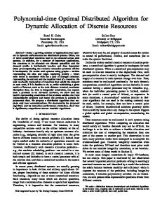
where DELETELO gives all partially redundant computations that can be eliminated profitably, COPYLO gives all computations that are not redundant themselves but cause other computations to be eliminated profitably, and INSERTLO gives all edge insertions required to make all partially redundant computations in DELETELO to become fully redundant. Such a simplification is not performed for MC-PREcomp since Lemma 4.7 does not hold for MC-PREcomp . The CMP-PRE algorithm we have implemented is described in [Bodik et al. 1998]. Given a CFG and a set of PRE candidate expressions in the CFG, CMP-PRE consists of solving three bit-vector data-flow problems simultaneously for all the candidate expressions and performing graph traversals on the CFG separately for these candidate expressions to identify their respective CMP (code-motion-preventing) regions. First, both availability and anticipatability analyses are performed on a CFG over a non-Boolean data-flow lattice with three values, MUST, MAY and NO. Second, the CFG is traversed, once for each PRE candidate expression (i.e., once for each PRE problem), to identify all CMP regions in the CFG. A CMP region for an expression π consists of all connected blocks such that π is both MAY-available and MAY-anticipatable (i.e., strictly partially available and anticipatable) on entry to each of its blocks. As a consequence, some entry edges to a CMP region are MUST-available (NO-available) in the sense that π is fully (not) available on exit from the source blocks of these edges. Similarly, some exit edges from a CMP region are MUST-anticipatable (NO-anticipatable) in the sense that π is fully (not) anticipatable on entry to the target blocks of these edges. Speculative PRE of π for a CMP region is profitable if the total execution frequency of MUST-anticipatable exit edges exceeds that of NO-available entry edges. In this case, hπ = π is inserted on all the NO-available entry edges to the CMP region. Third, availability analysis is re-run on the CFG. Finally, the CFG is transformed based on the information from the original anticipatability analysis and the new availability analysis. No specific algorithm was given in [Bodik et al. 1998] about how to find the CMP regions in a CFG. In our implementation, all CMP regions in a CFG for a PRE problem are found by using graph traversals of the CFG. 6.2 Experimental Setup Figure 6 depicts the GCC backend in which our algorithm is implemented and evaluated. The backend applies numerous passes to the RTL (Register Transfer Language) representation of a function, where the LCSE pass, i.e., the local PRE appears before the global PRE pass. Knoop, R¨ uthing and Steffen’s profile-independent LCM algorithm is the built-in global PRE pass, called GCSE, invoked at GCC’s O2 optimization level and above. 24
The LCM configuration shown represents exactly how GCC works when dynamic profiling is not explicitly enabled. In this case, GCC compiles a program only once. Due to the absence of dynamic profiling information, the “Branch Probabilities” pass works by predicting the branch probabilities statically. In our profile-guided framework, MC-PRE is the replacement for LCM. Due to the introduction of the “Edge Profiling” pass before MC-PRE, compiling a program requires GCC to be run twice. In the first run, we turn the switch “-profile-arcs” on so that GCC will instrument a program to gather its dynamic profiling information. The profiling information for all SPECcpu2000 benchmarks is always collected using the train input data sets. In the second run, we invoke GCC by turning the switch “-branch-probabilities” on. This instructs GCC to compute the edge profiles for all the functions in the program from the profiling information gathered in the first run. The edge profiling information can then be used by MC-PRE. In this second run, all benchmarks are executed using the reference input data sets. Immediately after the MC-PRE pass, we ignore the edge profiling information. There are two reasons for doing so. First, the GCC passes such as “Loop Optimization” and “CFG Optimization” as shown in Figure 6 do not update profiling information when performing some control flow restructuring transformations. This is because in GCC, the “Edge Profiling” pass is positioned after these passes and just before the “Branch Probabilities” pass. Such a phase ordering cannot be used for us since MC-PRE is profile-guided. Second, even if the profiling information is correctly updated, the “Branch Probabilities” pass will take advantage of this information to compute the branch probabilities, giving MC-PRE an unfair advantage over LCM. Like MC-PRE, MC-PREcomp and CMP-PRE are also profile-guided. Both are invoked in exactly the same way as MC-PRE as described above. In our experiments, all the four PRE algorithms use exactly the same set of PRE candidate expressions for a function. These are the expressions identified by GCC for its LCM pass. This way, we can have a fair evaluation about the relative strengths and weaknesses of the four PRE algorithms. In GCC, a PRE candidate expression is always the RHS of an assignment, where the LHS is a virtual register. The RHS expressions that are constants or virtual registers are excluded (since no computations are involved). So are any expressions such as call expressions with side effects. Therefore, all PRE candidate expressions are exception-free. (In our experiments, signed arithmetic is assumed to wrap around. This has often been the default option for C programs since signed overflow is undefined in C.) In all the PRE algorithms used, the same optimization passes are applied in exactly the same order. The only difference is that the “Edge Profiling” pass is needed to supply the edge profiles required by three speculative PRE algorithms, MC-PRE, MC-PREcomp and CMP-PRE. In addition, MC-PRE and MC-PREcomp use exactly the same bit-vector library used by LCM to perform their required data-flow analysis passes (for all distinct PRE candidate expressions in a CFG in parallel). CMP-PRE performs its data-flow analyses on the modified versions of these bit-vector routines since it works over a non-Boolean lattice. Note that the LCM configuration is the one from GCC 3.4.3. This provides an ideal setting for all the four PRE algorithms to compared against each other. 25
6.3 Redundancy Elimination and Performance Improvements One important criterion for measuring the effectiveness of a PRE algorithm is to quantify the number of non-fully redundant computations that it removes from a program. Figure 7 evaluates the four PRE algorithms using the SPECcpu2000 benchmarks according to this criterion. MC-PRE and MC-PREcomp are on par with each other since both are computationally optimal. LCM is the worst performer since it is profile-independent (and thus conservative). CMP-PRE is neither computationally optimal nor lifetime optimal. In principle, CMP-PRE lies between LCM and MC-PRE. MC-PRE eliminates more redundancies than both LCM and CMP-PRE in functions with complex control structures. As a result, the effectiveness of MC-PRE is more pronounced in SPECint2000 than in SPECfp2000. In the case of 12 SPECint2000 benchmarks, MC-PRE eliminates between 31.39% and 147.56% (an average of 90.13%) more non-full redundancies than LCM and between 0.28% and 58.76% (an average of 14.39%) more non-full redundancies than CMP-PRE. This has contributed to the performance improvements of MC-PRE over LCM and CMP-PRE in almost all its 12 benchmarks. In the case of 10 SPECfp2000 benchmarks, LCM has successfully eliminated over 80% of the nonfull redundancies in all the benchmarks except ammp. CMP-PRE has removed most of the remaining non-full redundancies from most of these benchmarks. However, the non-full redundancies that LCM and CMP-PRE fail to eliminate in a program can be from some of its hottest functions, and furthermore, these redundant computations can be occurrences of expensive PRE candidate expressions (e.g., memory operations) in these hottest functions. In these situations (as is the case for mesa and sixtrack), MC-PRE, which can eliminate all partial redundancies removable by using code motion and control speculation, can still achieve performance improvements in such programs over LCM and CMP-PRE. Figure 8 depicts the performance improvements (or degradations) of MC-PRE over MC-PREcomp , LCM and CMP-PRE. The execution time of a benchmark is taken as the arithmetic average of five runs and validated by the CPU cycles obtained using the pfmon tool available for the Itanium architecture. By removing more redundant computations and keeping the lifetimes of introduced temporaries to a minimum, MC-PRE can achieve nearly the same performance results as or better performance improvements than the other three algorithms in all 22 benchmarks. The performance degradations observed in some benchmarks are small. In general, MC-PRE improves the performance of a SPECint2000 benchmark over LCM and CMP-PRE due to the combined effects of optimizing a number of its hot functions. In the case of a SPECfp2000 benchmark, however, the performance improvement tends to come from optimizing fewer hot functions (typically one or two) in the benchmark. These results are analyzed in three separate sections below. 6.3.1 MC-PRE vs. MC-PREcomp . Figure 9 shows that MC-PREcomp introduces temporaries with longer lifetimes than MC-PRE. Recall that every computation of π removed by MC-PRE must also be removed by MC-PREcomp . The lifetime of hπ for a replacement computation (i.e., a use) of hπ in a CFG is measured to be the percentage of the basic blocks in which hπ is live in the CFG. Figure 5(a) compares MC-PRE and MC-PREcomp in terms of the average lifetimes of their introduced temporaries for non-isolated replacement computations (i.e., deletions) in 26
MC-PREcomp
CMP-PRE
ap si
art eq ua ke am mp six tra ck
wu pw ise sw im mg rid ap plu me sa
vp r gc c mc f cra fty pa rse r eo n pe rlb mk ga p vo rte x bz ip2 tw olf
Fig. 7.
Non-fully redundant computations eliminated (in dynamic terms).
MC-PREcomp
LCM
CMP-PRE
Fig. 8.
ap si
art eq ua ke am mp six tra ck
wu pw ise sw im mg rid ap plu me sa
ga p vo rte x bz ip2 tw olf
fty pa rse r eo n pe rlb mk
mc f
cra
vp r gc c
8 7 6 5 4 3 2 1 0 -1 gz ip
Speedups (%)
LCM
1 0.9 0.8 0.7 0.6 0.5 0.4 0.3 0.2 0.1 0 gz ip
Non-Full Redundancies Removed
MC-PRE
Percentage speedups of MC-PRE over MC-PREcomp , LCM and CMP-PRE.
a benchmark. The lifetimes for all benchmarks are longer under MC-PREcomp than MC-PRE. The percentage increases range between 17.97% for eon and 110.27% for ammp. Figure 5(b) depicts the lifetimes of temporaries for isolated computations that are introduced by MC-PREcomp but eliminated by MC-PRE. Comparing MC-PRE and MC-PREcomp in Figure 8, we see that minimizing the lifetimes of introduced temporaries certainly has an overall positive effect on performance. MC-PRE achieves the same or better performance results than MC-PREcomp in 19 out of the 22 benchmarks used. MC-PRE eliminates more redundancies than LCM and CMP-PRE and uses insertions with shorter lifetimes than MC-PREcomp . The combined effects of MC-PRE’s achieving both optimal results on performance will be examined below. 6.3.2 MC-PRE vs. LCM. As shown in Figure 8, MC-PRE achieves the same or better performance results than LCM in 19 out of 22 benchmarks. Some small performance losses are observed in wupwise, swim and applu. The benchmarks with better speedups are typically those in which MC-PRE has succeeded in eliminating more redundancies than LCM. These include gzip (3.63%), mcf (2.50%), crafty (2.69%), vortex (1.97%), bzip (2.04%) and twolf (1.37%) in the SPECint2000 benchmark suite and mesa (5.75%), art (1.64%) and sixtrack (7.03%) in the SPECfp2000 benchmark suite. By comparing MC-PRE and MC-PREcomp , we fur27
MC-PREcomp
ise swim mgri d applu m es a art equa ke am m p sixtr ack ap si
wup w
gzip
(a) Non-isolated deletions Fig. 9.
60 50 40 30 20 10 0 vp r g cc m cf craft y pars er eo n perlb mk g ap vorte x bzip 2 twolf
Lifetimes (%) ise swim mgri d applu m es a art equa ke am m p sixtr ack ap si
wup w
vp r g cc m cf craft y pars er eo n perlb mk g ap vorte x bzip 2 twolf
gzip
Lifetimes (%)
MC-PRE 60 50 40 30 20 10 0
(b) Isolated deletions by MC-PREcomp
Lifetimes of introduced temporaries by MC-PRE and MC-PREcomp .
ther observe that minimizing the lifetimes of introduced temporaries has generally contributed to the performance improvements in these benchmarks. MC-PRE tends to achieve the performance improvement in a SPECInt2000 benchmark by optimizing a number of its hot functions. For example, MC-PRE eliminates 100.84% more partial redundancies than LCM in crafty with 97.12% of these redundant computations coming from the following hottest functions in the benchmark: Evaluate, MakeMove, Search, UnMakeMove, GenerateCaptures, EvaluatePawns and NextMove. The performance improvements in these individual functions have contributed to the overall speedup of this benchmark. The two largest speedups, 5.75% and 7.03%, are attained in the two SPECfp2000 benchmarks, mesa and sixtrack, in which LCM has already removed the majority of their redundant computations. Both benchmarks serve as good examples to demonstrate the benefits for a PRE algorithm to achieve both computationally and lifetime optimal results in some programs. In both cases, the performance improvements (over LCM and CMP-PRE) are obtained because MC-PRE can achieve the two optimal results in one or two of their hot functions with complex control flow. In mesa, about 55.17% of the execution time from the compiled binary under LCM is spent on the three hottest functions, general textured triangle (21.50%), gl texture pixels (11.44%) and sample 1d linear (22.23%). MC-PRE removes only 19.55% more non-fully redundant computations than LCM (in dynamic terms). However, 94.7% of these are eliminated from sample 1d linear (whose CFG consists of 83 blocks and 119 edges). This represents 1.77% of the dynamic number of RTL instructions executed in the function. So the performance gain in mesa mostly comes from optimizing this function. Note that the minimization of lifetimes of introduced temporaries has also been beneficial (Figure 8). In sixtrack, the execution time from the compiled binary under LCM is mostly spent in its two hottest functions, thin6d (98.49%) and umlauf (0.93%). MC-PRE removes only 7.75% more non-fully redundant computations than LCM. However, all these redundant computations are removed from the two hottest functions: thin6d (52.01%) and umlauf (41.77%). Most of the performance gain comes from optimizing thin6d (with 196 blocks and 347 edges). Again Figure 8 shows clearly that the minimization of lifetimes of introduced temporaries has also contributed to the performance improvement in this benchmark. MC-PRE removes more redundancies than LCM. Despite this, the average lifetimes of introduced temporaries in both cases, as shown in Figure 10, are close. It is important to point out that LCM, which is profile-independent, is not computationally optimal for solving the speculative PRE problem. Therefore, LCM is not 28
MC-PRE
LCM
Lifetimes (%)
40 30 20 10
Fig. 10.
ap si
Lifetimes of introduced temporaries by MC-PRE and LCM.
9.00
Cycle Reductions (%)
art eq ua ke am mp six tra ck
pw ise sw im mg rid ap plu me sa wu
ip gz
vp r gc c mc f cra fty pa rse r eo n pe rlb mk ga p vo rte x bz ip2 tw olf
0
Unstalled Cycles
7.00
Front-end Flushes
5.00
GR Scoreboarding
3.00
FLP Stalls RSE Stalls
1.00
Instr Miss Stalls
-1.00
Branch Misprediction -3.00
D-cache Stalls apsi
ammp
sixtrack
art
equake
mesa
applu
swim
mgrid
wupwise
twolf
bzip2
gap
vortex
eon
perlbmk
parser
mcf
crafty
gcc
vpr
gzip
-5.00
Fig. 11. Performance improvements of MC-PRE over LCM split into those contributed by the individual reductions in the eight event categories. An event bar for a benchmark represents the performance speedup achieved by MC-PRE over LCM as a result of reducing the cycles in that event category. All the eight event bars for a benchmark add up to the performance speedup given in Figure 8 for that benchmark.
lifetime better than MC-PRE even though it achieves shorter lifetimes in a program than MC-PRE (Definition 3.8). With this caveat in mind, we see from Figure 10 that MC-PRE introduces temporaries with comparable lifetimes as LCM. Below we analyze the performance improvements of MC-PRE over LCM using pfmon. Figure 11 breaks down the performance speedup (or degradation) of a benchmark achieved by MC-PRE over LCM, which can be found in Figure 8, into eight components resulting from the corresponding cycle reductions (or increases) in the eight event categories. According to [Sverre Jarp 2002], the execution cycles of a program can be broken into stalls and unstalled cycles. The stalls can be further subdivided into seven categories: data cache (D-cache) stalls, branch misprediction, instruction miss stalls, register stack engine (RSE) stalls, floating-point unit (FLP) stalls, general register (GR) scoreboarding stalls and front-end flushes. As shown in Figure 11, MC-PRE has reduced the unstalled cycles in 16 out of the 22 benchmarks. The percentage reductions are particularly significant for gzip, mcf, bzip2, twolf and sixtrack, which are benchmarks with relatively large speedups. In the case of sixtrack, the one with the largest speedup, the decrease in its unstalled cycles has contributed to 84.34% of its performance improvement. 29
D-cache stalls and FLP unit stalls are known to be the main contributors to the pipeline stalls for integer and floating-point benchmarks in the SPECcpu2000 benchmark suite, respectively. D-cache stalls are mainly the bubbles caused by the latencies of integer load instructions while FLP unit stalls are the bubbles caused by the latencies of floating-point load instructions and inter-register dependencies. MC-PRE is applied only to the PRE candidate expressions that do not cause runtime exceptions. These include all RTL-level exception-free memory operations that may be eventually translated into loads. For example, (mem:m addr) represents one such a memory operation (i.e., access) at the address addr, where m specifies the smallest addressable unit for this memory operation. By eliminating more redundant computations – some of which are loads – than LCM, and by minimizing the lifetimes of introduced temporaries, MC-PRE has succeeded in reducing the D-cache stalls and FLP unit stalls in some benchmarks. However, since some of these redundant computations are eliminated speculatively, compensating insertions are made on the paths where those eliminated computations did not exist before. The D-cache and FLP unit stalls in some benchmarks are increased. Looking at all the benchmarks in Figure 11, we observe some relatively large reductions in the D-cache stalls in gap, mesa and sixtrack. On the other hand, mcf and equake suffer some visible increases. In the case of the SPECfp2000 benchmarks, we observe 3.81%, 2.91% and 3.84% reductions in terms of the FLP unit stalls for mesa, art and equake, respectively. In particular, mesa is the benchmark with the second largest speedup (5.75%). Some small increases in the FLP unit stalls are observed in wupwise, applu and sixtrack. If both D-cache and FLP unit stalls are combined, MC-PRE will be more effective than LCM in reducing the stall cycles in this combined category in 15 out of the 22 benchmarks. Figure 8 shows that MC-PRE results in slightly slower binaries than LCM in wupwise, swim and applu. In swim and applu, LCM has succeeded in removing almost all redundant computations. In wupwise, MC-PRE eliminates 16.62% more redundant computations than LCM with 99.04% of these redundancies being removed from zgemm, the hottest function in the benchmark. However, looking at Figure 11, the performance slowdowns in all three benchmarks are mainly caused by some slight increases in their FLP unit stall cycles. One challenging future work is to use a cost model that can also include a quantitative estimate of the impact of such an entity on performance to drive the PRE optimization. In summary, MC-PRE has reduced more unstalled cycles than LCM across most of the benchmarks used. In addition, the speculative elimination of safe memory operations (using temporaries with the shortest lifetimes as is possible) has an overall positive impact on reducing D-cache and FLP unit stalls. As shown in Figure 11, the decreases in these stall categories are responsible for the performance improvements achieved in the SPECcpu2000 benchmarks. 6.3.3 MC-PRE vs. CMP-PRE. All the four PRE algorithms can eliminate all fully redundant computations. MC-PRE removes optimally all non-fully redundant computations that can be removed by using speculative code motion. LCM can only remove some of these redundant computations non-speculatively. We measure the effectiveness of a speculative PRE algorithm by computing how much (in percentage) it can eliminate speculatively from all non-full redundancies that LCM fails to eliminate (non-speculatively). Figure 12 compares MC-PRE and CMP-PRE based 30
MC-PRE and CMP-PRE
80% 60% 40% 20%
i ap s
art eq ua ke am mp six tra ck
ap plu me sa
sw im mg rid
wu pw ise
tw olf
bz ip2
ga p vo rte x
eo n pe rlb mk
ty
er pa rs
mc f
cra f
vp r
gc c
0% gz ip
Non-Full Redundancies Removed Only Speculatively
MC-PRE 100%
Fig. 12. Non-fully redundant computations eliminated only speculatively by MC-PRE and CMP-PRE(i.e., these redundant computations cannot be eliminated by LCM).
CMP-PRE
30 20 10
Fig. 13.
ap si
art eq ua ke am mp six tra ck
pw ise sw im mg rid ap plu me sa wu
gz
ip
0 vp r gc c mc f cra fty pa rse r eo n pe rlb mk ga p vo rte x bz ip2 tw olf
Lifetimes (%)
MC-PRE 40
Lifetimes of introduced temporaries by MC-PRE and CMP-PRE.
on this criterion. The problem of finding computationally optimal transformations is a min-cut problem. MC-PRE finds required insertion edges optimally while CMP-PRE restricts its search to the NO-available entry edges to CMP regions. In general, MC-PRE eliminates more redundancies than CMP-PRE for CFGs with complex control structures. In the case of SPECint2000, MC-PRE eliminates between 0.52% and 280.47% (an average of 58.15%) more partial redundancies that are only speculatively removable than CMP-PRE. In the case of SPECfp2000, the percentage increases range from 0.00% to 89.98% with an average of 15.23%. CMP-PRE is more effective in SPECfp2000 than in SPECint2000. This is because, as shown in Figure 7, LCM itself (with no speculation) has successfully eliminated over 80% of all partial redundancies in nine out of its 10 benchmarks. Figure 13 shows that CMP-PRE uses temporaries with slightly longer lifetimes in 17 out of the 22 benchmarks (even though it is not computationally optimal). By eliminating more redundant computations and using temporaries with shorter lifetimes, MC-PRE achieves the same or better performance results than CMP-PRE in 19 out of the 22 benchmarks as shown in Figure 8. Let us look at the three benchmarks, crafty, mesa and sixtrack, that we examined previously in Section 6.3.2. For crafty, we mentioned earlier that MC-PRE eliminates more partially redundant computations than LCM from its hottest functions: Evaluate, MakeMove, Search, UnMakeMove, GenerateCaptures, EvaluatePawns and NextMove. As shown in Figures 7 and 12, of all non-fully redundant computations that cannot be removed by LCM but are completely removed by MC-PRE, CMP-PRE has eliminated only 31
Unstalled Cycles
7.00
Front-end Flushes
5.00
GR Scoreboarding
3.00
FLP Stalls
1.00
RSE Stalls Instr Miss Stalls
-1.00
Branch Misprediction -3.00
Fig. 14.
apsi
ammp
sixtrack
art
equake
mesa
applu
swim
mgrid
wupwise
twolf
bzip2
gap
vortex
eon
perlbmk
parser
mcf
crafty
gzip
vpr
D-cache Stalls -5.00
gcc
Cycle Reductions (%)
9.00
Performance improvements of MC-PRE over CMP-PRE.
26.28% of these redundant computations. In particular, search is the only function for which CMP-PRE has successfully removed all its partially redundant computations. So the performance improvements from optimizing these individual functions have again resulted in the overall speedup of this benchmark. Let us now take a look at mesa, the benchmark for which MC-PRE achieves the largest speedup over CMP-PRE. As we discussed in Section 6.3.2, MC-PRE eliminates almost all nonfull redundancies that LCM fails to eliminate in its hot function sample 1d linear. Figure 12 shows that only 66.67% of these redundant computations are removed by CMP-PRE. Furthermore, MC-PRE has eliminated more redundant computations statically than CMP-PRE and LCM. LCM removes eight partially (fully or nonfully) redundant computations from eight distinct expressions. CMP-PRE eliminates seven more partially redundant computations all from two new expressions. However, all these operations removed by LCM and CMP-PRE are arithmetic. MC-PRE has removed 41 more non-fully redundant computations from these existing expressions and 12 new ones on memory access, sign-extension, shift and compare. This has resulted in the actual performance improvements of MC-PRE over LCM and CMP-PRE. In sixtrack, we mentioned in Section 6.3.2 that among all speculatively removable redundancies that are removed by MC-PRE, 93% are from its two hottest functions: thin6d (52.01%) and umlauf (41.77%). CMP-PRE has eliminated all these speculatively removable redundancies from thin6d but nothing at all from umlauf. Since thin6d consumes the most of the execution time in this benchmark, MC-PRE achieves only some slight performance improvement over CMP-PRE. Figure 14 gives an analogue of Figure 11 for CMP-PRE. As in the case of LCM, the performance improvements of MC-PRE over CMP-PRE are generally obtained from the cycles reductions in the same three stall categories, namely, unstalled cycles, D-cache stalls and FLP unit stalls. Some small performance losses are observed in twolf and wupwise due to slightly increases in D-cache stalls and FLP unit stall and applu due to more branch mispredictions introduced. In summary, MC-PRE can optimally exploit more optimization opportunities in programs than a non-optimal algorithm like CMP-PRE. In the case when MC-PRE is more effective than CMP-PRE in hot functions, which may have complex control flow, in a program, some performance improvement is often expected. 32
MC-PREcomp
LCM
CMP-PRE
1.1 1.05 1 0.95
Fig. 15.
ap si
art eq ua ke am mp six tra ck
sw im mg rid ap plu me sa
wu pw ise
olf
ip2
tw
bz
ga p vo rte x
mc f cra fty pa rse r eo n pe rlb mk
ip
vp r gc c
0.9 gz
Normalized Static Sizes
MC-PRE
Static code sizes.
6.4 Static Code Sizes Figure 15 compares the static code sizes of all benchmarks (normalized to MC-PRE) compiled under the four PRE algorithms. The size of a compiled benchmark is taken as the size of the text section of its binary obtained using the UNIX command size as suggested in [Beszedes 2003]. A PRE algorithm both inserts and deletes computations. So it may cause some benchmarks to expand and others to shrink in their code sizes. All four PRE algorithms are comparable in terms of this size criterion except that MC-PREcomp results in slightly larger binaries (particularly in the case of wupwise and applu). MC-PREcomp makes insertions and deletions for isolated computations. As a result, the increases in code size are observed in 19 out of the 22 benchmarks. The overall increase of MC-PREcomp over MC-PRE for all benchmarks is 1.43%. By comparing LCM and MC-PRE, we find that MC-PRE has caused small code size expansions in only six out of the 22 benchmarks with an overall size increase of 0.78%. Finally, CMP-PRE has resulted in slightly smaller binaries than MC-PRE in 12 out of the 22 benchmarks. However, the overall increase of MC-PRE over CMP-PRE for all 22 benchmarks is only 0.50%. 6.5 Compile Times Figure 16 gives the compile times of GCC in compiling all benchmarks under the four PRE algorithms. All compile times are normalized with respect to MC-PRE. MC-PREcomp is generally more expensive than MC-PRE due to some unnecessary insertions and deletions MC-PREcomp introduces for isolated computations. CMP-PRE is generally more expensive than LCM. This is partly because CMP-PRE performs three bit-vector data-flow analyses over a non-Boolean lattice and partly because CMP-PRE also needs to traverse a CFG separately for each distinct PRE problem in order to identify its CMP regions. The compile times of MC-PRE are slightly larger than CMP-PRE in some benchmarks but smaller in others. In comparison with LCM, the extra compilation overheads MC-PRE pays for achieving the performance improvements in all the benchmarks are relatively small. In the case of SPECint2000 benchmarks, the compile-time increases for gcc, crafty and perlbmk are 4.50%, 8.72% and 3.63%, respectively. The increases of less than 1.86% are observed in the remaining nine benchmarks. In the case of SPECfp2000, the worst three benchmarks are wupwise, equake and sixtrack. Their compile-time increases are 4.37%, 5.05% and 9.22%, respectively. Each of the remaining seven 33
MC-PREcomp
LCM
CMP-PRE
1.05 1 0.95
Fig. 16.
art eq ua ke am mp six tra ck ap si
Compile times.
CFGs
EFGs
600.00 500.00 400.00 300.00 200.00 100.00 art eq ua ke am mp six tra ck ap si
wu pw ise sw im mg rid ap plu me sa
vp r gc c mc f cra fty pa rse r eo n pe rlb mk ga p vo rte x bz ip2 tw olf
0.00 gz ip
Average Sizes of PRE Problems
wu pw ise sw im mg rid ap plu me sa
ga p vo rte x bz ip2 tw olf
eo n pe rlb mk
fty pa rse r
mc f
cra
vp r
gc c
0.9 gz ip
Normalized Compile Times
MC-PRE 1.1
Fig. 17. Average sizes of PRE problems on CFGs and EFGs. Given a CFG, distinct PRE candidate expressions in the CFG result in distinct PRE problems. The empty EFGs are excluded in calculating the average number of blocks per EFG (which would be much smaller otherwise).
Empty
Nonempty
100% 80% 60% 40% 20%
Fig. 18.
i ap s
rac k six t
e
p am m
eq ua k
a
art
me s
ap plu
sw im
mg rid
wu pw ise
tw olf
bz ip2
ga p
vo rte x
eo n pe rlb mk
pa rs
er
ty cra f
mc f
gc c
vp r
gz ip
0%
Empty v.s. nonempty reduced graphs (or EFGs).
benchmarks has a compile-time increase of less than 1.85%. Finally, of all the 22 benchmarks, seven compile even slightly faster under MC-PRE than LCM. There are two reasons why MC-PRE is only slightly more expensive than LCM. First, Figure 17 shows that the EFGs are significantly smaller than the original CFGs across all the benchmarks. Given an EFG Gst = (Nst , Est , W pst ), finding a minimum cut for it using Goldberg’s HIPR algorithm takes O(|Nst |2 |Est |) [Goldberg 2003]. Transforming CFGs to their smaller EFGs has reduced the cost of the algorithm significantly. Furthermore, as shown in Figure 18, the reduced graphs for the majority of the PRE problems in nearly all benchmarks are empty. This 34
means that the corresponding EFGs are also empty. The minimum cut for an empty EFG is empty, requiring no invocation to a min-cut algorithm in our implementation (as discussed in Section 6.1). (By Lemma 4.1, if the EFG for a PRE problem is empty, then all redundancies (if any) must be full redundancies and are all removed by MC-PRE.) Second, nonempty EFGs are constructed efficiently. We have modified GCC’s edge def struct so that a single traversal of a CFG in Step 3.4 of MC-PREcomp is sufficient to produce the corresponding nonempty EFG. Le us investigate why the seven benchmarks, vpr, bzip2, swim, mgrid, applu, art and apsi, as shown in Figure 8, compile slightly faster under MC-PRE than LCM. These seven benchmarks contain in that order 17828, 5191, 1067, 1600, 7603, 2147 and 15490 PRE problems to be solved, respectively. LCM performs PRE by conducting each of the four data-flow analysis passes in parallel on these PRE problems. On the other hand, MC-PRE first applies two data-flow analysis passes on these problems in parallel to reduce them into smaller PRE problems on EFGs. As a result, these seven benchmarks have in that order only 4327, 1213, 188, 234, 845, 532 and 2947 nonempty EFGs, which are the PRE problems that require the min-cut step of MC-PRE to be invoked. These nonempty EFGs are rather small (with 9.77 blocks for vpr, 5.19 blocks for bzip2, 2.75 blocks for swim, 2.21 blocks for mgrid, 3.50 blocks for applu, 5.42 blocks for art and 9.14 for apsi on the average). So the min-cut step completes very quickly. Then MC-PRE performs a third data-flow analysis on all original PRE problems in parallel to avoid insertions and deletions for isolated computations. Therefore, MC-PRE can compile a program faster than LCM if a large number of PRE problems in the program have empty EFGs (which require only three data-flow analysis passes) and if the nonempty EFGs are small (so that the min-cut step completes quickly). Finally, we examine why MC-PRE is not so much more costly than LCM in the worst case. As shown in Figure 8, crafty and sixtrack are the two most expensive benchmarks to compile. Figure 19 plots the histograms of all the nonempty EFGs for the two benchmarks according to their sizes. Although crafty has some relatively large EFGs, 92.46% of them have fewer than 300 blocks. On the other hand, sixtrack has more large EFGs. There are 80.02% EFGs with fewer than 300 blocks. In the remaining EFGs, there are 1510 with 300 – 999 blocks, 1098 with 1000 – 1999 blocks and 996 with more than 1999 blocks. However, Figure 18 shows that in sixtrack, 85.37% of EFGs are empty. Due to the first two reasons given above and the fact that the efficiency of the min-cut algorithm used, the compile time increase of MC-PRE over LCM in this worst-case benchmark is only 9.22%. 7. CONCLUSION We have presented the first lifetime optimal algorithm, MC-PRE, that performs speculative PRE by combining code motion and control speculation. We have proved rigorously the optimality of this algorithm. MC-PRE works for the CFGs consisting of standard basic blocks so that it can be readily implemented by researchers in a compiler framework. The algorithm is conceptually simple since it is centered around three standard bit-vector data-flow analyses and a standard mincut algorithm. We have implemented MC-PRE, and consequently, MC-PREcomp in GCC 3.4.3. For comparison purposes, we have also implemented CMP-PRE, a previously reported non-optimal speculative PRE algorithm [Bodik et al. 1998], in GCC 35
Number of Nonempty EFGs
Cumulative %
1400 1200 1000 800 600 400 200 0
Number of Nonempty EFGs
100.00% 80.00% 60.00% 40.00% 20.00%
100.00% 80.00% 60.00% 40.00% 20.00% 0.00% 1-99 100-2 99 300-5 99 600-8 99 900-9 99 1000 -129 9 1300 -159 9 1600 -189 9 1900 -199 9 >= 2 000
>=50 0
9
9 100-1 49 150-1 99 200-2 99 300-3 99 400-4 99
50-9
5-9
10-4
1-4
0.00%
Number of Blocks
Number of Blocks
(a) crafty
(b) sixtrack
Fig. 19.
Cumulative %
14000 12000 10000 8000 6000 4000 2000 0
Nonempty EFGs of crafty and sixtrack.
3.4.3. We have evaluated MC-PRE against MC-PREcomp , LCM and CMP-PRE using the 22 C, C++ and FORTRAN 77 benchmarks in SPECcpu2000 on Itanium 2. Our experimental results show that MC-PRE is capable of eliminating more partial redundancies than both LCM and CMP-PRE and always uses temporaries with shorter lifetimes than MC-PREcomp . Achieving both computationally and lifetime optimal results in a program allows MC-PRE to explore more optimization opportunities, particularly in its functions with complex control structures. This has led to the performance improvements in almost all of these benchmarks over the other three algorithms at the costs of small compile-time and code-size increases in some benchmark programs. As profile-guided compiler optimizations are becoming increasingly more aggressive, more sophisticated algorithms will likely be employed in future compile systems. In addition to the PRE optimization as discussed in this paper, the min-cut algorithm has also been recently used in decomposing a sequential program into speculatively parallel threads [Johnson et al. 2004]. Finally, we want to stress that PRE techniques are applicable to other areas of optimisation such as load/store elimination by combining both control and data speculation [Lin et al. 2003], load/store elimination for binaries [Fern´ andez and Espasa 2004], communication optimisation [Knoop and Mehofer 2002], and threadlevel synchronisation cost elimination [Zhai et al. 2002]. Significant performance gains can be expected from these optimisations, leveraging the benefits of a more application-specific PRE technique that may be derived from our algorithm. Furthermore, our algorithm may find applications in some embedded applications [Scholz et al. 2004] where performance improvements can be beneficial. One future work is to evolve MC-PRE into a more application-specific PRE technique in these research areas so that more significant performance gains can be obtained. 8. ACKNOWLEDGEMENTS We wish to thank the reviewers and editors for their helpful comments and suggestions. This work is partially supported by an ARC grant DP0452623. REFERENCES Alpern, B., Wegman, M. N., and Zadeck, F. K. 1988. Detecting equality of variables in programs. In Proceedings of the 15th ACM SIGPLAN-SIGACT Symposium on Principles of
36
Programming Languages. 1–11. Beszedes, A. 2003. Optimizing for space: Measurements and possibilities for improvement. In GCC Summit 2003. Bodik, R. 1999. Path-sensitive value-flow optimizations of programs. Ph.D. thesis, University of Pittsburgh. Bodik, R., Gupta, R., and Soffa, M. L. 1998. Complete removal of redundant computations. In Proceedings of the ACM SIGPLAN ’98 Conference on Programming Language Design and Implementation. 1–14. Briggs, P. and Cooper, K. D. 1994. Effective partial redundancy elimination. In Proceedings of the ACM SIGPLAN ’94 Conference on Programming Language Design and Implementation. 159–170. Cai, Q. and Xue, J. 2003. Optimal and efficient speculation-based partial redundancy elimination. In 1st IEEE/ACM International Symposium on Code Generation and Optimization. 91–104. Chang, P. P., Mahlke, S. A., Chen, W. Y., Warter, N. J., and mei W. Hwu, W. 1991. Impact: An architectural framework for multiple-instruction-issue processors. In Proceedings of the 18th Annual International Symposium on Computer Architecture. 266–275. Chekuri, C., Goldberg, A. V., Karger, D. R., Levine, M. S., and Stein, C. 1997. Experimental study of minimum cut algorithms. In Proceedings of the Eighth Annual ACM-SIAM Symposium on Discrete Algorithms. 324–333. Chow, F. 1983. A portable machine-independent global optimizer — design and measurements. Ph.D. thesis, Computer Systems Laboratory, Stanford University. Click, C. 1995. Global code motion / global value numbering. In Proceedings of the ACM SIGPLAN’95 Conference on Programming Language Design and Implementation (PLDI). 246– 257. Cormen, T. H., Leiserson, C. E., and Rivest, R. L. 1990. Introduction to Algorithms. Cambridge, Mass.: MIT Press. Cytron, R., Ferrante, J., Rosen, B. K., Wegman, M. N., and Zadeck, F. K. 1991. Efficiently computing static single assignment form and the control dependence graph. ACM Trans. Program. Lang. Syst. 13, 4, 451–490. Dhamdhere, D. M. 1991. Practical adaptation of the global optimization algorithm of Morel and Renvoise. ACM Trans. Program. Lang. Syst. 13, 2, 291–294. Dhamdhere, D. M., Rosen, B. K., and Zadeck, F. K. 1992. How to analyze large programs efficiently and informatively. In Proceedings of the ACM SIGPLAN’92 Conference on Programming Language Design and Implementation (PLDI). 212–223. Drechsler, K.-H. and Stadel, M. P. 1993. A variation on Knoop, R¨ uthing, and Steffen’s lazy code motion. SIGPLAN Notices 28, 5, 29–38. ´ndez, M. and Espasa, R. 2004. Link-time path-sensitive memory redundancy elimination. Ferna In International Conference on High-Performance Computer Architecture. 300–310. Ford, L. R. and Fulkerson, D. R. 1962. Flows in Networks. Princeton University Press. Goldberg, A. 2003. Network Optimization Library. http://www.avglab.com/andrew/soft.html. Gupta, R., Berson, D. A., and Fang, J. Z. 1998. Path profile guided partial redundancy elimination using speculation. In Proceedings of the 1998 International Conference on Computer Languages. 230–239. Hailperin, M. 1998. Cost-optimal code motion. ACM Transactions on Programming Languages and Systems 20, 6, 1297 – 1322. Horspool, R. and Ho, H. 1997. Partial redundancy elimination driven by a cost-benefit analysis. In 8th Israeli Conference on Computer System and Software Engineering. 111–118. Hosking, A. L., Nystrom, N., Whitlock, D., Cutts, Q. I., and Diwan, A. 2001. Partial redundancy elimination for access path expressions. Softw., Pract. Exper. 31, 6, 577–600. Hu, T. C. 1970. Integer Programming and Network Flows. Addison-Wesley. Johnson, T. A., Eigenmann, R., and Vijaykumar, T. N. 2004. Min-cut program decomposition for thread-level speculation. SIGPLAN Not. 39, 6, 59–70.
37
Kennedy, K. 1972. Safety of code motion. International Journal of Computer Mathematics 3, 2– 3, 117–130. Kennedy, R., Chan, S., Liu, S.-M., Lo, R., and Tu, P. 1999. Partial redundancy elimination in SSA form. ACM Transactions on Programming Languages and Systems 21, 3, 627–676. Kennedy, R., Chow, F. C., Dahl, P., Liu, S.-M., Lo, R., and Streich, M. 1998. Strength reduction via SSAPRE. In Proceedings of the 7th International Conference on Compiler Construction. Springer-Verlag, London, UK, 144–158. Knoop, J. 1998. Optimal interprocedural program optimization: A new framework and its application. Number 1428 in LNCS. Knoop, J., Collard, J.-F., and Ju, R. D.-C. 2000. Partial redundancy elimination on predicated code. In Proceedings of the 7th Static Analysis Symposium (SAS’00). 260–279. Knoop, J. and Mehofer, E. 2002. Distribution assignment placement: Effective optimization of redistribution costs. IEEE Trans. Parallel Distrib. Syst. 13, 6, 628–647. ¨thing, O., and Steffen, B. 1992. Lazy code motion. In Proceedings of the ACM Knoop, J., Ru SIGPLAN ’92 Conference on Programming Language Design and Implementation. 224–234. ¨thing, O., and Steffen, B. 1994. Optimal code motion: Theory and practice. Knoop, J., Ru ACM Trans. Program. Lang. Syst. 16, 4, 1117–1155. Lin, J., Chen, T., Hsu, W.-C., Yew, P.-C., Ju, R. D.-C., Ngai, T.-F., and Chan, S. 2003. A compiler framework for speculative analysis and optimizations. In Proceedings of the ACM SIGPLAN ’03 Conference on Programming Language Design and Implementation. 289–299. Lo, R., Chow, F., Kennedy, R., Liu, S.-M., and Tu, P. 1998. Register promotion by sparse partial redundancy elimination of loads and stores. SIGPLAN Not. 33, 5, 26–37. Morel, E. and Renvoise, C. 1979. Global optimization by suppression of partial redundancies. Commun. ACM 22, 2, 96–103. Morgan, R. 1998. Building an Optimizing Compiler. Butterworth-Heinemann. Muchnick, S. S. 1997. Advanced Compiler Design and Implementation. Morgan Kaufmann Publishers, Inc. Rosen, B. K., Wegman, M. N., and Zadeck, F. K. 1988. Global value numbers and redundant computations. In Proceedings of the 15th ACM SIGPLAN-SIGACT Symposium on Principles of Programming Languages. 12–27. ¨thing, O., Knoop, J., and Steffen, B. 2000. Sparse code motion. In Conference Record of the Ru 27th Annual ACM SIGPLAN-SIGACT Symposium on Principles of Programming Languages (Boston, Massachusetts). ACM, New York, 170 – 183. Scholz, B., Horspool, R. N., and Knoop, J. 2004. Optimizing for space and time usage with speculative partial redundancy elimination. In Proceedings of the 2004 ACM SIGPLAN/SIGBED Conference on Languages, Compilers, and Tools for Embedded Systems. 221– 230. Simpson, L. T. 1996. Value-driven redundancy elimination. Ph.D. thesis, Rice University. Steffen, B. 1996. Property-oriented expansion. In Proceedings of the 3rd Static Analysis Symposium (SAS’96). Lecture Notes in Computer Science, vol. 1145. Springer-Verlag, Heidelberg, Germany, 22 – 41. ¨thing, O. 1990. The value flow graph: a program representation Steffen, B., Knoop, J., and Ru for optimal program transformations. In Proceedings of the third European symposium on programming on ESOP ’90. Springer-Verlag New York, Inc., New York, NY, USA, 389–405. ¨thing, O. 1991. Efficient code motion and an adaption to Steffen, B., Knoop, J., and Ru strength reduction. In TAPSOFT ’91: Proceedings of the international joint conference on theory and practice of software development on Advances in distributed computing (ADC) and colloquium on combining paradigms for software development (CCPSD): Vol. 2. SpringerVerlag New York, Inc., New York, NY, USA, 394–415. Sverre Jarp. 2002. A methodology for using the Itanium 2 performance counters for bottleneck analysis. http://www.gelato.org/pdf/Performance counters final.pdf. Zhai, A., Colohan, C. B., Steffan, J. G., and Mowry, T. C. 2002. Compiler optimization of scalar value communication between speculative threads. In ASPLOS-X: Proceedings of
38
the 10th International Conference on Architectural Support for Programming Languages and Operating Systems. ACM Press, 171–183.
39