A HMM-BASED METHOD FOR RECOGNIZING DYNAMIC VIDEO CONTENTS FROM TRAJECTORIES A. Hervieu1 , P. Bouthemy1 and J-P. Le Cadre2 IRISA / INRIA Rennes, 2 IRISA / CNRS Campus Universitaire de Beaulieu, F-35042 Rennes cedex, France 1
ABSTRACT This paper describes an original method for classifying object motion trajectories in video sequences in order to recognize dynamic events. Similarities between trajectories are expressed from Hidden Markov Models representing each trajectory. We have favorably compared our method to several other ones, including histogram comparison, Longest Common Subsequence distance and SVM classification. Trajectory features are computed from the curvature and velocity values at each point of the trajectory, so that they are invariant to translation, rotation and scale. We have evaluated our method on two sets of data, a first one composed of typical classes of synthetic trajectories (such as parabola or clothoid), and a second one formed with trajectories obtained by tracking cars in a Formula1 race video. Index Terms— Image sequence analysis, Image motion analysis, Hidden Markov models, Pattern classification. 1. INTRODUCTION Object tracking is now mature enough so that it is possible to get reliable and accurate moving object trajectories in various situations. These trajectories are usually given as sequences of consecutive positions in a 2D space (the image plane (x,y)). Investigations on their semantic analysis are growing, since such data may help recognizing events, actions, or interactions between objects. The aim is also to provide rich information required for automatic video monitoring or exploitation (video surveillance, sports video analysis,...)[1]. Several methods have been developed to classify trajectories from video sequences. Buzan et al. [2] resorted to the Longest Common Subsequence (LCSS) distance to classify trajectories computed in an image sequence acquired by a single stationary camera for video surveillance. It is based on a hierarchical unsupervised clustering of trajectories represented by the set of 2D trajectory points coordinates. Systems performing trajectory clustering and abnormal event detection were developed by Hu et al. [3], where a first clustering stage is performed based on spatial information, and a second one exploits temporal information. Bashir et al. [4] introduced two trajectory classification methods inspired by speech analysis, especially one splitting trajectories into pieces using cur-
vature information, and then classifying trajectories based on a HMM framework applied to the successive subtrajectories. Naftel et al. also performed trajectory clustering and abnormal event detection by modeling trajectories using orthogonal basis function representations, clustering being carried out in the chosen feature space [5]. F. Porikli designed a HMMbased method involving a translation and scale factor invariant feature [6]. These methods exploit features that are not simultaneously invariant to translation, rotation and scale transformation. Also most previous work on trajectory classification and clustering amounts to form groups of similar trajectories (often exploiting explicit scene structure information). Our approach is to treat any trajectory (of any length) and to extract classes that correspond to similar movements in terms of intrinsic trajectory shape and object speed, without any knowledge of the scene structure and without any camera calibration. Therefore, to classify trajectories, we propose trajectory features invariant to translation, rotation and scale; and a recognition method based on HMM to capture the time evolution of the viewed dynamic event. In Section 2, we present the translation, rotation and scale invariant feature we have considered. In Section 3, we describe our HMM-based comparison method for trajectories. In Section 4, we introduce other classification methods to be compared to the HMM-based one. In Section 5, we first comment the two data sets used to test the methods, the second one being formed by trajectories extracted from real videos of a Formula 1 race. Results are then reported and discussed. 2. TRAJECTORY FEATURE EXTRACTION In video analysis and interpretation, invariance to different transformations is required : translation, rotation and scale at least must be considered. It may be helpful in a wide range of video applications. 2.1. Kernel approximation We suppose that a trajectory Ti is defined by a set of n points corresponding to the successive positions of the tracked object in the image sequence, we note Ti = {(x1 , y1 ), .., (xn , yn )}. Before computing the trajectory features, which are differential values, it is preferable to have a continuous representation
of the curve formed by the trajectory. To this end, we compute a kernel approximation of Ti defined by : PN −( t−j )2 PN −( t−j )2 h h xj yj j=1 e j=1 e ut = P N PN −( t−j )2 . t−j 2 , vt = −( ) h h j=1 e j=1 e
divided into a given number N of bins (in Fig. 1 a histogram corresponding to a trajectory of the sinusoid class in [-S, S]). For every trajectory, the histogram will be bounded to [-S, S] and evaluated with the same number of bins.
Such a representation will allow us to explicitly derive expressions for the first and second order temporal derivatives of u and v, u˙ t , v˙ t , u ¨t and v¨t , and a Gaussian kernel is an usual and convenient choice. 2.2. Invariant features Most of the video trajectories clustering methods developed so far use trajectory coordinates ut and vt as input features. These coordinates are helpful to study spatial resemblance between trajectories, but our approach is more to consider the overall shape of trajectories than their exact instances. First, taking into account the successive local orientations of the trajectories is more attractive and it helps comparing the overall shape of the trajectories. If we consider γ = arctan( uv˙˙ ) value, we have a translation and scale invariant feature value. γt ) = cos12 γt γ˙ t . Let us now consider γ˙ t . We have d(tan dt On the other hand, we can write: d(tan γt ) v¨t u˙ t − u ¨t v˙ t = . dt u˙ 2t � � v¨t u˙ t − u ¨t v˙ t Then . γ˙ t = cos2 γt u˙ 2t u˙ 2 Also cos2 γt = (1 + tan2 γt )−1 = 2 t 2 . u˙ t + v˙ t Finally, we get γ˙ t = where κt = and kwt k =
v¨t u˙ t − u ¨t v˙ t = κt .kwt k 2 u˙ t + v˙ t2
v ¨t u˙ t −¨ ut v˙ t 3
is the local curvature of the trajectory
(u˙ 2t +v˙ t2 ) 2 1 (u˙ 2t + v˙ t2 ) 2
the local point (ut , vt ). The � speed of � v¨t v˙ t is a determinant numerator v¨t u˙ t − u ¨t v˙ t = det u ¨t u˙ t and then is rotation invariant. The denominator u˙ 2t + v˙ t2 is the square of the speed and is rotation invariant, then γ˙ t is rotation invariant. Since γt is translation and scale invariant, as a consequence γ˙ t is translation, scale and rotation invariant. The feature vector considered to represent a given trajectory is then the vector containing the successive values of γ˙ t : V = [γ˙ 1 , γ˙ 2 , ..., γ˙ n−1 , γ˙ n ]. 3. TRAJECTORY SIMILARITY AND CLASSIFICATION 3.1. Hidden Markov model approach To model the distribution of γ, ˙ we first focus on an interval containing a given percentage P of measured γ˙ values (for the entire set of trajectories to classify) in order to eliminate the “outlier” measurements and maintaining the Markov chains states to a bounded and representative number. Then [-S, S] is
Fig. 1. Example of a normalized histogram (histogram of a trajec-
tory of the sinusoid class) with h = 3, P = 90 (see text), and N = 31 (number of bins).
We then turn toward an additional information, i.e., the temporal transitions between γ˙ values. A usual tool to account for this is the Markov chains framework. A Markov chain with N states, is characterized by : - the state transition matrix A = {aij } with aij = P [ qt+1 = Sj | qt = Si ], 1 ≤ i, j ≤ N. where Si corresponds to the state index i, and qt is the state at time t. - the initial state distribution π = {πi }, where πi = P [ q1 = Si ], 1 ≤ i ≤ N. In our setup, we associate the states with the histogram bins, and each trajectory is associated with a Markov chain. However, some aij could be hard to train (for example, for a small trajectory, there will be few observations, and several histogram values could be empty). This would lead to infinite distance measures between Markov chains representing different trajectories. To avoid such configurations, we turn toward an original discrete HMM. We now consider that the states qt are hidden and the HMM is characterized by the triplet (A, B, π) where B is composed of conditional observation probabilities B = {bj (γ˙ t )}, with bj (γ˙ t ) = P [γ˙ t | qt = Sj ], where qt is the unknown hidden state at time t. For the conditional observation probability bi (γ˙ t ), we adopt a Gaussian distribution of mean µi (given by the median value of the histogram bin Si ). Its standard deviation σ is specified so that the interval [µi − σ, µi + σ] corresponds to the bin width (therefore, it does not depend on the state for an uniform quantization). This conditional observation model can reasonably account for measurement uncertainty. It will also prevent from having zero values when estimating matrix A in the training stage by lack of measures. We have adapted the least-squares technique introduced in [7] to estimate A and Π, where the HMM is assimilated to (i) a count process. If we denote Ht = P (γ˙ t |qt = i) (i.e., a weight for the count process), empirical estimates of A and Π, for a trajectory of size M are given by
aij =
(i) (j) n=1 Hn Hn+1 PM −1 (i) n=1 Hn
PM −1
and πi =
PM
n=1
Hni
M
.
3.2. Similarity measure and classification The distance used to compare two HMMs associated to two trajectories is the one proposed by Rabiner [8]. Given two HMMs, λ1 and λ2 (λi = (Ai , Bi , πi ), i = 1, 2), we consider 1 D(λ1 , λ2 ) = [log P (O(2) |λ2 ) − log P (O(2) |λ1 )] T and the symmetrized version is : 1 Ds (λ1 , λ2 ) = [D(λ1 , λ2 ) + D(λ2 , λ1 )]. 2 where O(j) = γ˙ 1 γ˙ 2 ...γ˙ T is the sequence of states corresponding to Tj knowing λj (estimated using a Viterbi algorithm) and P (O(j) |λi ) expresses the probability of observing O (j) with model λi . To define the distance between a trajectory Ti and a class of trajectories Gj , we use the average link technique by computing the mean of the distance of Ti to all trajectories Tlj in Gj : P Tlj ∈Gj Ds (Ti , Tlj ) Daverage link (Ti , Gj ) = . #Gj Classification is then performed by assigning the processed trajectory to the nearest class. 4. OTHER APPROACHES TO BE COMPARED 4.1. Bhattacharyya distance between histograms
5. EXPERIMENTS 5.1. Synthetic trajectories First, to test the designed method, we have generated a set of typical trajectories. More specifically, we have considered 8 classes (sinusoid, parabola, hyperbola, ellipse, cycloid, spiral, line and clothoid) and we have simulated 8 different trajectories for each class, corresponding to different parametrization of the curves, and for several geometric transformations (rotation, scaling) (Fig. 2).
Fig. 2. Plots of one synthetic trajectory for four classes. 5.2. Video trajectories We have also processed real trajectories extracted from a Formula1 race TV program filmed with several cameras. The trajectories are computed with a tracking method based on optical flow calculated on interest points. The background motion due to camera panning, zooming and tilt is canceled (as plotted on Fig. 3 and 4).The trajectories supplied by this method are then very similar to the real 3D trajectories of the cars (up to an homography, since the 3D motion is plane).
To demonstrate the importance of introducing temporal causality, i.e., transitions between bins, we have implemented a Bhattacharyya distance-based classification method. The Bhattacharyya distance Db between two (normalized) histograms hi and hj is defined as : N q X Db (hi , hj ) = 1 − hki hkj k=1
where hki
is the histogram value of bin k for trajectory i. Similarly to the HMM-based method, we assign the test trajectory to the nearest class and the distance to a class is defined using an average link method (see subsection 3.2). 4.2. SVM classification method
Fig. 3. Images from video shots acquired by two different cameras at two different places on the circuit. The computed trajectories are overprinted on the images.
An efficient tool to classify patterns is SVM [9]. As input for SVM, we take the HMM parameters corresponding to the trajectories. SVM need patterns to be represented by vectors. Hence, for each trajectory, we create a vector containing the corresponding HMM parameters. For example, let us consider the HMM λi corresponding to the trajectory Ti (for convenience, we develop an example with only N = 3) such that 1 0 a11 Ai = @ a21 a31
a12 a22 a32
a13 a23 A , πi = [a1 a2 a3 ]. a33
Xi = [a11 a12 a13 a21 a22 a23 a31 a32 a33 a1 a2 a3 ] will be the vector characterizing trajectory Ti . We use a SVM classification technique with a Gaussian Radial Basis Function kernel. The reported results are obtained using the “one against all” classification scheme.
Fig. 4. Plots of the 10 classes of dynamic content (trajectories) for a Formula1 race video, each box contains a different class. A class of trajectories is composed of trajectories extracted from shots acquired by the same camera. The different classes correspond to different cameras placed throughout the circuit at different strategic turns.
5.3. Experimental results We have compared our HMM-based method with the SVM classification, the technique based on the Bhattacharyya distance and the LCSS distance based one. To evaluate the performances, we have adopted the leave-one-out cross validation for a wide range of values for h (smoothing parameter in the curve approximation step), P (percentage of data considered to specify [-S, S]) and N (number of states). By adding noise to the simulated trajectories, we can evaluate the influence of the h parameter value. Classification results with noised data shows that the parameter h helps handling efficiently noised data, by smoothing the processed trajectories. A high value is required for highly corrupted data (Table 1). Tests performed on the sets of synthetic trajectories gave very promising results, hence a perfect classification was performed for most parameter configurations (i.e., for N , h and Pv ) with the SVM and HMM methods, while the technique based on the Bhattacharyya distance fails to efficiently classify synthetic trajectories (highlighting the importance of the temporal causalities modeled with HMM). The technique based on the Longest Common Subsequence distance (LCSS) [2] gave good results but not perfect, and with a higher computation time (more than five times longer than with HMM based method). For the evaluation on real videos, four cases were considered: 4, 6, 8 and 10 classes, the group of 4, 6 and 8 classes being nested subsets of the ten ones presented in Fig.4. Quite satisfactory classification results were obtained for most parameter configurations with the SVM and HMM methods, while the techniques based on the Bhattacharyya distance and the LCSS distance provide less accurate classification results (Table 2). Our HMM based method gave better results than the SVM method, showing the importance of the Viterbi algorithm used to compute the Rabiner distance between HMMs. Besides, our HMM method is much more flexible than the SVM classification stage (e.g., adding a new class only requires to learn the parameters of that class). Best classification results are obtained when P is set to 95%. The choice of the number of states N is less straightforward to fix. For some configurations, considering few states gives best results, and for other ones, a higher N (30 to 50) gives better results.
Table 2. Comparison of the best recognition percentages for the trajectories extracted from real video, using the leave-one-out cross validation technique.
6. CONCLUSION We have proposed a HMM-based method to classify video events. Extracted trajectories of moving objects are adequate image primitives to characterize dynamic contents, and we have defined appropriate trajectory features invariant to translation, rotation and scale transformations. By comparing the designed method to other ways of tackling this problem, we have justified the choice of these features and of a HMMbased classification scheme. Very promising results on synthetic and real examples have been obtained. We are carrying out additional experiments on real videos to further assess the performances of the method. 7. REFERENCES [1] A. Kokaram, N. Rea, R. Dahyot, M. Tekalp, P. Bouthemy, P. Gros, and I. Sezan, “Browsing sports video (trends in sportsrelated indexing and retrieval work),” IEEE Trans. Signal Processing, vol. 23, no. 2, pp. 47–58, March 2006. [2] D. Buzan, S. Sclaroff, and G. Kollios, “Extraction and clustering of motion trajectories in video,” in Proc. of the 17th Int. Conf. Pattern Recognition, Cambridge, UK, Aug. 2004, pp. 521–524. [3] W. Hu, X. Xiao, D. Xie, T. Tan, and S. Maybank, “A system for learning statistical motion patterns,” IEEE Trans. Pattern Anal. Machine Intell., vol. 28, no. 9, pp. 1450–1464, Sept. 2006. [4] F.I. Bashir, A. A. Khokhar, and D. Schonfeld, “View-invariant motion trajectory-based activity classification and recognition,” ACM Multimedia Systems, vol. 12, no. 1, pp. 45–54, 2006. [5] A. Naftel and S. Khalid, “Classifying spatiotemporal object trajectories using unsupervised learning in the coefficient feature space,” ACM Multimedia Systems, vol. 12, no. 3, pp. 227–238, 2006. [6] F. Porikli, “Trajectory distance metric using hidden markov model based representation,” in Eur. Conf. Computer Vision, PETS Workshop, Prague, Czech Republic, May 2004. [7] J. Ford and J. Moore, “Adaptive estimation of HMM transition probabilities,” IEEE Trans. Signal Processing, vol. 46, no. 5, pp. 1374–1385, 1998.
Table 1. Classification results for the synthetic trajectories, with a HMM-based method, using the leave-one-out cross validation technique, for different values of h and σ (σ is the standard deviation of the added noise).
[8] L. Rabiner, “A tutorial on hidden markov models and selected applications in speech recognition,” Proc. IEEE, vol. 77, no. 2, pp. 257–285, 1989. [9] C. Burges, “A tutorial on support vector machines for pattern recognition,” Data Mining and Knowledge Discovery, vol. 2, pp. 121–167, 1998.