A fast heuristic Cartesian space motion planning algorithm for many-DoF robotic manipulators in dynamic environments Phuong D.H. Nguyen, Matej Hoffmann, Ugo Pattacini, and Giorgio Metta Abstract— A variety of motion planning algorithms has been developed over the past decades. For robotics, the transformation of the problem from the robot Cartesian space (workspace) to the configuration space (C-space) has been crucial—converting the problem of collision-checking between 3D objects to simpler, point-like, tests in the high-dimensional C-space. However, the C-space map-making is both computationally and memory-intensive and the complexity grows with the C-space dimension. With time-varying environments and many robot DoFs, this soon becomes intractable, as newly appearing and possibly moving obstacles need to be remapped online into the high-dimensional C-space. Therefore, we present a fast heuristic planning method designed for a humanoid robot that employs the sampling-based RRT* algorithm directly in the Cartesian space and in a hierarchical fashion: first, a collision-free path is planned for the end-effector; second, corresponding collision-free points for every via-point are searched for the robot elbow. The resulting path consists of straight-line segments and is only approximate, but the details— a kinematically feasible smooth trajectory for the robot—is offloaded to an online Cartesian solver and controller that is available on our platform. The results demonstrate, first, that our solution delivers real-time performance (plans faster than 1s on a standard PC) in the vast majority of cases in a significantly cluttered environment. Second, the results are suggestive of the fact that asymptotic optimality of the plans is preserved even for the additional control points. Third, a test of state-of-the-art algorithms on the same scenario shows that solutions cannot be found in reasonable time (less than 10s).
I. INTRODUCTION AND RELATED WORK The problem of motion planning is relevant in different disciplines (in particular artificial intelligence, robotics, and control theory) and in many application areas such as machining using numerically controlled tools, assembly, or robot motion planning, including both mobile robots and manipulators (see e.g., [1]). The problem consists in finding a collision-free path for a rigid object in an environment containing other rigid objects (obstacles), connecting start and goal configuration and possibly respecting other constraints and optimizing certain criteria (such as length of the path). In its generality, the path planning problem is almost intractable [2]. In practice, efficient and even complete1 This work was supported by the European Union Seventh Framework Programme project WYSIWYD (FP7-ICT-612139). M.H. was supported by a Marie Curie Intra-European Fellowship (iCub Body Schema 625727). P.N. was supported by a Marie Curie Early Stage Researcher Fellowship (H2020MSCA-ITA, SECURE 642667) P. Nguyen, M. Hoffmann, U. Pattacini, and G. Metta are with iCub Facility, Istituto Italiano di Tecnologia, Via Morego 30, 16123 Genova, Italy. {phuong.nguyen, matej.hoffmann,
ugo.pattacini, giorgio.metta}@iit.it 1 An algorithm is considered complete if for any input it correctly reports whether there is a solution in a finite amount of time.
solutions can be found depending on the problem at hand. Considering the classical “piano-moving” type of problems, the difficulty consists primarily in how the collision-checking in the Cartesian space (or workspace) is performed. For reasons of computational efficiency, the 2D or 3D objects (robot and obstacles) need to be approximated by more simple objects such as polytopes (polygons in 2D, polyhedra in 3D; e.g. [3]); yet, this step will still be computationally expensive. Here, the introduction of configuration space (Cspace) representation has been fundamental [4]: the complete robot configuration is described as a single point in this, typically higher-dimensional, space (with dimensionality corresponding to the number of robot degrees of freedom – DoF). The obstacles are then remapped into the same space, forming regions (C-space obstacle) in which the obstacles collide with the body of the robot in the particular configuration. After this transformation, collision free paths for the robot can be searched more easily in this space and complete and optimal2 algorithms exist (they are sometimes referred to as exact motion planning algorithms; see e.g. Ch. 2 in [1]). In practice, the exact transformation of obstacles from the workspace into the configuration space is often intractable or even theoretically impossible [5]. Also real-time performance is desirable. Barraquand et al. [6] presented a technique that performs faster by connecting local minima of potential fields in the C-space. More recently, sampling-based motion planning algorithms have become very popular, which trade absolute completeness and optimality for probabilistic completeness and asymptotic optimality. Sampling is performed in the robot configuration space and the points sampled are mapped into workspace and checked for collisions with obstacles. As mentioned above, the collision checking becomes a primary computational bottleneck of these approaches, which has motivated modifications of the approach to warrant more favorable computational complexity (most recently [5]). Finally, the resulting plan may undergo—often also computationally costly—postprocessing such as interpolation and smoothing. The output of this stage is a smooth collisionfree path in configuration space that can be transformed into a trajectory (which includes the temporal dimension) to command the robot in joint space. However, our setting is quite different. We are seeking a solution for reaching in a humanoid robot (the iCub [7]) in a dynamic environment and using existing Cartesian solvers and controllers available for the robot [8]. An example is 2 returning
the shortest path
shown in Fig. 1 – the scene may be cluttered and humans may also constitute dynamic obstacles. Thus, guaranteeing collision-free trajectory execution at all times will not be feasible and is not our goal. Instead, our requirement on the planner is to obtain an approximate collision free-path for the hand and arm of the robot in real time. Then, we will rely on other layers of our architecture (not the subject of this article) to ensure safe interaction of the robot with its environment. These are: (i) local avoidance reflexes for the whole robot body triggered by a safety margin (peripersonal space) representation [9]; (ii) responses to collision on contact relying on the artificial pressure-sensitive skin and Force/Torque sensors mounted on the robot. Similar frameworks were presented by [10], [11], for example.
recruited. Given this context, we developed a relatively simple planner that matches these requirements. The basic component is an RRT* sampling-based motion planner in the 3D workspace to obtain the path for the robot end-effector. The robot reachable space is simply superimposed onto the workspace; the obstacles are represented with polyhedra and collision-checking with the robot end-point can be done very fast using inequalities only. However, the collision-free plan for the end-effector does not suffice—we want to consider the whole body. At the same time, we want to avoid representing the whole body of the robot using meshes or polyhedra as this would render the collision checking much more difficult. Therefore, we have introduced a coarse but effective approximation to consider the forearm occupancy: we include the elbow and the forearm midpoint into the planning problem. The planner is then applied hierarchically—for every two via points of the end-effector, RRT* is triggered to provide a corresponding local plan for the forearm midpoint. Finally, the elbow is checked for collisions with obstacles too (somewhat similarly to [12]). The article is structured as follows. In Section II, overall framework, the algorithm proposed, and the experimental setup are described. This is followed by Results and finally Conclusion, Discussion, and Future Work. II. METHODS AND EXPERIMENTAL SETUP A. Overview of overall control architecture
Fig. 1: Illustration of scenario in the robot. The scene may be cluttered and moving obstacles (including humans) may be present. Thus, the key characteristics of our scenario and their implications for the planning problem are: 1) The obstacles may appear and disappear dynamically and be even moving. This precludes their mapping into C-space and also renders any caching of their positions w.r.t. the robot (such as the safety certificates introduced in [5]) less efficient. 2) The output of the planner needs to be only coarse— a sequence of via points in workspace connected by straight lines. A smooth trajectory in joint space (with the minimum-jerk property) will be a result of the application of the Cartesian solver and controller to the via points. 3) The redundancy of the manipulator is not part of the planning problem (which happens in workspace), but will be taken care of by the Cartesian solver. 4) The number of DoFs available to the robot may change dynamically – there will be 7 arm joints employed; in addition 1-3 torso joints (pitch, roll, yaw) may be
A schematics of our overall framework is shown in Fig. 2. The central node, “Multiple-Cartesian-point planner” is the subject of this article. However, the context of the other modules is essential to understand its working principle. In short, the planner provides a service—a path for several points on the manipulator—when queried by the supervisor, which in turn relays this information to a solver and a controller that can handle multiple Cartesian points. The planner has direct access to the perceptual module to locate the goal and obstacles in the workspace as well as to the “kinematic chain” to retrieve the current robot configuration, using forward kinematics, and the starting position for the control points. Objects (Target, Obstacles..)
Control points position planning request user's request
paths of the Control points
References of Control points
Fig. 2: Overview of overall control framework. 1) “Perception”: Interfaces to various modules available for the YARP (Yet Another Robot Platform) [13] [14]
2)
3)
4)
5)
and iCub software repositories that deal with 3D object segmentation and tracking, relying on stereoscopy from the robot’s two cameras (e.g., [15], [16]). These can be used to stream current positions of both target and obstacles in the scene. “Kinematic chain” provides the position of all control points on the robot: end-effector, midpoint of forearm, and elbow by applying forward kinematics to the current configuration of the robot. “Multiple-Cartesian-point planner”: This module uses information about target and obstacles and the current state of control points as input and generates collisionfree motion paths for all control points, composed of via points connected by straight lines. The details of the algorithm will be described in Section II-C. “Supervisor”: This module receives a planning request from the user (human or another module) and forwards it to the planner. Then, after receiving the motion paths from the planner, it uses simple linear interpolation to create a trajectory (reference points in time) in Cartesian space that is in turn forwarded to the multiple Cartesian point solver and controller. “Multiple-Cartesian-point controller” is an extension of the Cartesian inverse kinematics solver and controller [8] that can accommodate multiple control points and both solver and controller are combined into a single optimization problem in velocity space, using the IPOPT library [17].
B. RRT* algorithm RRT (Rapidly-exploring Random Tree) algorithm [1] is one of the most common incremental sampling-based algorithms for robotics, which generates a path connecting the initial state and goal state by randomly growing a search tree. It is probabilistically complete but most of the time converges to a non-optimal solution, which is why RRT* [18] was introduced. RRT* introduces a cost function (e.g Euclidean distance between vertices in the tree) to guide the extension of new vertices of the tree in such a way that the algorithm can find a shortest path. While its computational complexity is only a constant factor of RRT, it is also asymptotically optimal—guaranteed to converge to an optimal solution as the number of samples approaches infinity. Perez et al. [19] have further augmented the algorithm with a sparse sampling procedure. C. Multiple Cartesian point planning algorithm The main idea of the Cartesian planning algorithm proposed here is to use individual (modular) planners in the workspace for a few selected control points on the manipulator. Imagine taking the End-Effector (EE) and the Elbow (EB) as control points. At first, the planner of the EE may use the information from the environment (target and obstacles) and EE’s position to generate a collision-free motion path for the EE only. Based on this path, local planners for the next control point, the elbow, can be applied to find collision free paths for the elbow for every segment of the end-effector’s
path. Yet, there is a problem with this approach, as illustrated schematically in a 2D scenario in Fig. 3a. According to the new position of the End-Effector at EE’, the local planner of the Elbow can find a new position for it at EB’ so that both paths are free of collision. However, the occupancy of the forearm (wrist-elbow link) has not been taken into account, which may lead to collisions with small obstacles on the course. Thus, we introduce a new control point in the middle of the link (MP), leading to for example the situation in Fig. 3b. This may still not guarantee a collision-free path in every case, but in most situations and given the size of obstacles our robot will encounter, it is a good enough approximation. The algorithm proposed is hierarchical and modular in nature: First, a plan (a set of via points connected by straight lines) is generated for the end-effector. Then, for every segment of this path, local collision-free paths are searched for the forearm midpoint. Finally, a check for collisions with the elbow is also performed. If it is not possible to construct a collision-free plan for all the control points, re-planning from the top (end-effector) is triggered. The details of the algorithm are described in pseudo-code in Algorithm 1. Algorithm 1 Multiple Cartesian point planning Algorithm 1: 2: 3: 4: 5: 6: 7: 8: 9: 10: 11: 12: 13: 14: 15: 16: 17: 18: 19: 20: 21: 22: 23: 24: 25: 26: 27: 28: 29: 30:
EST IMAT E −WORKSPACE UPDAT E − MANIPULAT OR − POSE OBTAIN − SCENE repeat clear(EE − path) while (!EE − path) do MODULAR − PLANNER(EE, EE − pos, GOAL) end while if (end − e f f ector − path) then for all wi ∈ (EE − path) do DILAT E − OBSTACLE(wi ) end for repeat i=0 sMP = MP − pos repeat PICK −V IAPOINT (wi , wi+1 ) gMP = goalMP ← wi+1 MODULAR − PLANNER(MP, sMP , gMP ) if (size(MP − path) > 2) then sucess ← PAD −V IAPOINT (EE) end if i ← i+1 sMP = gMP until size(EE − path) = size(MP − path) FIND − ELBOW sucess ← CHECK −COLLISION − ELBOW until (!EB − collisions) end if until (success)
The key components of the algorithm are explained below. All coordinates are w.r.t. Root Frame of Reference of the
EE MP
EE MP
EE'
EB
EB
MP'
EB' EB'
EB'
MP'
EE'
MP'
(a)
EE'
EB''
(b)
(c)
MP''
EE''
Fig. 3: Schematics of a 2 DoF planar manipulator with obstacles (red) and target (green). (a) Part of a plan for End-Effector and elbow (EB) illustraing that a collision-free path for the two control points does not guarantee that no collisions will occur for the whole manipulator occupancy (b) Introduction of another control point in the forearm link helps to avoid collisions, eventually leading to collision-free path from start to goal as shown in c).
iCub (Root FoR), located around its waist. • ESTIMATE–WORKSPACE uses an inverse kinematics solver (using IPOPT library) to estimate the reachable space for the end-effector, as visualized in Fig. 4. This procedure is computationally expensive but can be precomputed offline. A corresponding approximation of the reachable space of the forearm midpoint is derived by simply shrinking the end-effector reachable space by a constant corresponding to EE-MP distance. This automatically guarantees compliance with the kinematic constraints: for far away targets, the elbow will naturally assume poses “inside”—between the torso and the endeffector. • UPDATE–MANIPULATOR–POSE uses forward kinematics at the current joint configuration (3 torso joints and 7 arm joints) to calculate the position of the endeffector and the elbow and then infers the position of the forearm midpoint (see Fig. 5). • OBTAIN–SCENE retrieves information about objects, i.e position and size, from corresponding perceptual modules. The coordinates are converted to iCub Root FoR in the process. • MODULAR–PLANNER(control point, start, goal) applies the RRT* algorithm to generate a free of collision path from “start” to “end”. This can be a global plan in case we deal with the end-effector, or a local plan that seeks the forearm midpoint positions corresponding to two end-effector via points. • DILATE–OBSTACLE(via point) dilates the size of all obstacles which are close to each via point of the previous control point’s motion path, as illustrated in Fig. 6. Only obstacles (red) inside the area swept by the wrist-midpoint (EE-MP) link, namely obstacles 1, 2, 4 and 5, are dilated. For the case of the forearm midpoint planning, obstacles will be dilated w.r.t. to the via points of the End-Effector path. This procedure prevents midpoint’s local planners to generate unfeasible paths or via points. • PICK–VIAPOINT(wi ,wi+1 ) obtains two successive via points (wi ,wi+1 ) of the generated path of the previous control point—end-effector in case of planning for
•
•
•
forearm midpoint. These via points are then used as starting and ending position for the modular planner, using fixed geometric relations between the end-effector and forearm link. PAD–VIAPOINT(control point, via point position) is used to generate additional via points in a top-level path if triggered by the lower-level modular planner. As illustrated in Fig. 6, the presence of obstacle 3 requires the creation of an additional via point (MP”) for the forearm midpoint. To warrant equal number of via points for all control points, the top-level (end-effector) path needs to be “padded” with an additional via point (EE”). FIND–ELBOW computes the set of the elbow’s positions corresponding to the (end-effector, midpoint) pairs (the via points in the already constructed plans), as determined by the forearm geometry. CHECK–COLLISION–ELBOW examines whether the new generated path (and all via points) of the elbow is collision-free.
Fig. 4: Visualization of the reachable space of the left arm of iCub, starting from the Root FoR in the robot’s waist area. The color map depicts the manipulability of the different poses. D. Experimental setup
YARP platform
Perception
ROS platform
Objects (Target, Obstacles..)
Controlled points position
Multiple-Cartesianpoint Planner
Kinematic Chain
YARPROS messages
planning ack
planning request
Fig. 7: Communication between YARP and ROS for scenario synchronization.
Fig. 5: Schematics of the kinematic chain of iCub – left arm and torso. Reference frames have their z-axes labeled. The 0th reference frame is the iCub Root; the last (“z10 ”) corresponds to the end-effector. dilated obstacles
2
4 EE
1
EE'' EE'
(URDF) 4 file from the CAD design files of iCub, and then use the Setup Assistant tool provided by MoveIt! to generate MoveIt! compatible ROS packages which can be called by MoveIt! during run-time (see [21] for details). Fig. 7 shows the communication mechanism between the iCub simulator in YARP environment and iCub simulator in the ROS-MoveIt! environment. The connection is used to synchronize scenarios between the 2 simulators for the comparison of planning performance. 2) The cost function: In our experiments, the cost is defined as the total motion distance for a path of a representative point as in Equation 1. In particular, the representative points in our scenarios are the end-effector and the elbow.
MP''
MP
3
N−1
MP'
cost path =
5
∑ ||wi − wi+1 ||
(1)
i=0
Fig. 6: 2D illustration of DILATE-OBSTACLES and PADVIAPOINT. See text for details.
1) Robot and Simulator: The iCub robot [7] (shown in Fig. 1) is a humanoid robot composed of 38 DoFs for the upper body, 3 DoFs for the torso, and 6 DoFs for each leg. This research focuses only on using 7 DoFs of the arm (3 shoulder joints, 2 elbow joints, 2 wrist joints) and 3 DoFs of the torso. A physics-based simulator of the robot [20] is also available (see Fig. 8). ROS 3 (Robot Operating System) is an open-source robotics software framework, which has been developing broadly with the contribution of robotics community. MoveIt! [21] is a robotics software library implemented in ROS environment, which provides tools like motion planning, manipulation, 3D perception, kinematics, control and navigation. Particularly, MoveIt! use the Open Motion Planning Library (OMPL, [22]) as the core for the motion planning model, providing many different sampling-based planners, namely RRT*, PRM*, RRTConnect, etc. We will use this motion planning environment to benchmark the performance of our algorithm. In order to simulate the iCub robot in ROS-MoveIt! environment, we obtain the Unified Robot Description Format 3 http://www.ros.org/
where: (a) wi , wi+1 are successive via points on the path; (b) N is number of via points on the path; (c) ||.|| is the Euclidean distance calculation between 2 via points 3) Experiments: The experimental scenario is shown in Fig. 8: the goal is to construct a motion plan for the robot to reach an object, the target, on a table (tabletop scenario), while avoiding other objects as obstacles. While the target is fixed, the position of all obstacles are randomly changed for every trial in such a way that they do not overlap with the target. The default number of generated obstacles is 10 but if a generated obstacle is placed at the target position, the obstacle will be omitted. Thus the number of obstacles on the table is variable. The obstacles are slightly taller than the target, but a collision-free plan still always exists because the robot can reach for the target from top. However, such a plan will have a higher cost than approaching from the side. All the experiments were run on a standard PC (Processors: 4 × Intel Core i5-4310U CPU 2.00GHz, graphics: Intel Haswell Mobile, RAM: 8Gbs, OS: Ubuntu 14.04LTS 64-bit). Hence, the planning times reported in the Results section are referring to this PC. 4 http://wiki.ros.org/urdf
III. RESULTS Three types of experiments were conducted. First, we conducted a batch experiment with the maximum allowed planning time for individual planners fixed and we studied the performance statistics in 1000 randomly generated environments. Second, we kept the environment fixed and varied the maximum planning time to investigate the asymptotic optimality of the planner. Finally, we compared some characteristics of our planner performance with state-of-the-art planners.
PERCENTAGE OF TRIALS (%)
80
73.50
0.54 0.52 0.5 0.48 0.46 0.44 0.1
0.3
0.5
0.7
0.9
1.1
1.3
1.5
MAX TIME FOR SINGLE MODULAR PLANNER (s) 0.7
ELBOW COST (m)
Fig. 8: Experimental scenario with iCub simulator, target (green), randomly generated obstacles (red), and motion plans for end-effector (blue), forearm midpoint (yellow), and elbow (violet).
END-EFFECTOR COST(m)
fixed the time any of these modular planners can take to 0.1s. However, the number of calls to the individual planners is not known in advance and depends on the environment: the number of via points is determined dynamically by the planner. Furthermore, if the local planners for forearm midpoint or the final elbow collision checking fails, replanning from the top-level is triggered. Thus, the total computation time is the sum of all the individual planners’ execution. The bar graph in Fig. 9 summarizes the results of the batch experiment in terms of this total planning time. It shows that 73.50% of trials complete with computation time of less than half of second, and 18.80% trials finish with from 0.5s to 1s of computation time. The percentage for computation time form 1s to 2s is 5.5%. In summary, a majority of trials (97.8%) can finish within 2s, which is suitable for our setting. The fact that all percentages sum up to 100% confirms that a solution was found in all cases.
0.65 0.6 0.55 0.5 0.45 0.4 0.1
0.3
0.5
0.7
0.9
1.1
1.3
1.5
MAX TIME FOR SINGLE MODULAR PLANNER (s)
Fig. 10: Cost of control point as a function of the defined planning time of modular planners (horizontal axis). The vertical bars show the standard deviation over 50 trial while the stars indicate the mean values of motion cost. Top: endeffector; Bottom: elbow.
60
40
18.80
20
B. Asymptotic optimality experiments
5.50 1.40
0.20
0.60
2s-5s
5s-10s
>10s
0 <0.5s
0.5s-1s
1s-2s
TOTAL PLANNING TIME (s)
Fig. 9: Summary of a batch experiment with 1000 trials. A. Run-time batch experiment In this experiment, 1000 trials were conducted successively one-by-one with new randomly generated obstacle positions. As explained in Section II-C, the algorithm proposed has a hierarchical structure and involves a series of calls to individual “modular” planners. In these experiments, we
For this experiment, the obstacles are randomly created, but their positions kept unchanged from then on. Here, the timeout for every individual planner is systematically varied: after every 50 trials, the planning time is increased by 0.2 s. After each trial, the planning results, namely total computation time and cost of motion plan (see Section IID.2), are stored. The experiments are finished when the simulator completes all 50 trials at the setting of 1.5s timeout for each modular planner. The results in Fig. 10 indicate that the motion costs reduce when the modular planning time is increased, for both of 2 representative points of the forearm (end-effector and elbow). Please note that only the
end-effector uses a unique global planner (RRT*) while the elbow path (calculated through the forearm midpoint) is a result of application of local planners to the end-effector via points. Yet, the results suggest that the asymptotic optimality of the original RRT* algorithm is transferred to the additional control points. A formal proof will, however, remain the subject of future work. C. Comparison with state-of-the art C-space algorithms Using the setup with OMPL and MoveIt! as explained in Section II-D.1, we aimed at comparing our results with state-of-the-art planners available through the OMPL library. For every trial of this experiment, information about all obstacles is synchronized to ROS-MoveIt! module to update the environment. Then, different motion planning algorithms (RRT*, PRM* and RRTConnect) are applied to the new scenario, with maximum computation time set to 10s. When the whole planning computation in ROS-MoveIt! finishes, there is an acknowledgment sent back to our planner in YARP environment (as displayed in Fig. 7) to allow the planner to start a new trial (our planner running with 0.1s timeout for individual planners as in Section III-A). The planning results of our algorithm and OMPL-provided algorithms are stored for comparison. The results in terms of total computation time as well as cost spoke in favor of our algorithm. However, we are aware that this comparison would not be fair, as our algorithm solves a much easier problem in a heuristic fashion (using only a very simplified Cartesian space representation for the planning and collision checking) and offloads a number of expensive steps to the other modules (trajectory generation, smoothing, inverse kinematics and control of robot in joint space). Conversely, the C-space planners deal with a complete representation of the robot geometry and provide a collision-free, smooth trajectory that is kinematically feasible. Nonetheless, the most important implication from our results is that with the 10s time-out, RRT*, PRM* and RRTConnect delivered a successful solution only in 11.93%, 9.17% and 8.26% cases respectively—while our algorithm in 100% cases, with average total planning time of 0.454s, 0.440s and 0.411s, respectively. Thus, the standard C-space planners cannot be deployed in our scenario where real-time response is required. IV. CONCLUSION, DISCUSSION, FUTURE WORK We presented a motion planning component that is designed to work as part of a control framework for a humanoid robot that is reaching in a cluttered, dynamically changing environment. Moreover, the overall framework contains additional control layers to guarantee the robot’s as well as the environment’s safety by relying on an artificial pressuresensitive skin as well as force/torque sensing. Thus, a perfect, collision-free plan is not a requirement; instead, we were seeking a module that delivers approximate collision-free paths very fast. Given the high number of robot DoF (7 arm joints and 3 torso joints) and the fact that the obstacles may not be static, we realized that standard configuration space
planning solutions cannot cope with this scenario. For example, [23] survey configuration space mapping techniques, but none of the manipulators reviewed feature more than 6 DoF. Therefore, we devised a solution that employs standard RRT* sampling-based algorithm, but directly in the Cartesian space (workspace) to construct a collision-free path for the end-effector. In order to consider the occupancy of the robot body as well, we used a collection of heuristics. Only the robot forearm was considered in addition to the end-point and the planner was modified to operate in a hierarchical, modular fashion: local planners were launched to seek plans for the control points on the forearm, such that they match with the via points obtained for the end-effector. Collisionchecking is very simple and fast, through inequalities in the worskpace and employing a simple heuristics to dilate obstacles when considering the forearm midpoint path. The results demonstrate, first, that our solution delivers realtime performance (plans faster than 1s on a standard PC) in the vast majority of cases in a significantly cluttered environment. Second, the results are suggestive of the fact that asymptotic optimality of the plans is preserved even for the additional control points. Third, a test of state-of-the-art algorithms on the same scenario shows that solutions cannot be found in reasonable time (<10s). With respect to the last result (comparison with C-space algorithms), it has to be clearly stated that our method is solving a much easier problem. In a way, it is transforming planning for a many-DoF manipulator with kinematic constraints to the case of a mobile robot moving in 3D space. The fact that we are dealing with a manipulator is re-introduced through additional heuristics adding the forearm occupancy. However, these approximation do not guarantee a collision-free path in all cases. Furthermore, the inverse kinematics problem and the generation of smooth, kinematically feasible trajectories is also not dealt with— it is offloaded to Cartesian solvers and controllers that are available on our platform (and are also proven to cope with real-time requirements). We are considering a number of improvements for our future work. First, our algorithm was empirically found to deliver the desired real-time performance. The complexity of the plain algorithm should scale roughly linearly with the number of control points in moderately cluttered spaces, however, the hierachical, recursive-like structure does not provide any guarantees on the maximum planning time (frequent replanning may be triggered in highly cluttered environments). Here the efficiency of our proposed solution can be improved in the future: in case that it is not possible to find a collision-free path for the forearm and elbow—given the existing plan for the end-effector—the end-effector planning is started anew. However, the tree already constructed for the end-effector can be profitably recycled. Third, the asymptotic optimality of our solution was suggested only empirically— this needs to be addressed in the future. Finally, the overall control framework—of which the planning module is only one component—needs to be tested on the real robot.
ACKNOWLEDGMENT
[12]
We’d like to thank Alessandro Roncone for support with the iCub reachable space computation and visualization. R EFERENCES [1]
[2] [3]
[4]
[5]
[6]
[7]
[8]
[9]
[10]
[11]
S. M. LaValle, Planning Algorithms. Cambridge, U.K.: Cambridge University Press, 2006, Available at http://planning.cs.uiuc.edu/. J. H. Reif, Complexity of the generalized mover’s problem. 1985. E. G. Gilbert, D. W. Johnson, and S. S. Keerthi, “A fast procedure for computing the distance between complex objects in three-dimensional space,” IEEE Journal on Robotics and Automation, vol. 4, no. 2, pp. 193–203, Apr. 1988. T. Lozano-Perez, “Spatial planning: a configuration space approach,” IEEE transactions on computers, vol. 100, no. 2, pp. 108–120, 1983. J. Bialkowski, M. Otte, S. Karaman, and E. Frazzoli, “Efficient collision checking in sampling-based motion planning via safety certificates,” The International Journal of Robotics Research, vol. 35, no. 7, pp. 767– 796, Jun. 1, 2016. J. Barraquand, B. Langlois, and J.-C. Latombe, “Numerical potential field techniques for robot path planning,” IEEE Transactions on Systems, Man, and Cybernetics, vol. 22, no. 2, pp. 224–241, 1992. G. Metta, L. Natale, F. Nori, G. Sandini, D. Vernon, L. Fadiga, C. Von Hofsten, K. Rosander, M. Lopes, J. Santos-Victor, and others, “The iCub humanoid robot: an open-systems platform for research in cognitive development,” Neural Networks, vol. 23, no. 8, pp. 1125–1134, 2010. U. Pattacini, F. Nori, L. Natale, G. Metta, and G. Sandini, “An experimental evaluation of a novel minimum-jerk cartesian controller for humanoid robots,” in Intelligent Robots and Systems (IROS), 2010 IEEE/RSJ International Conference on, IEEE, 2010, pp. 1668–1674. A. Roncone, M. Hoffmann, U. Pattacini, and G. Metta, “Learning peripersonal space representation through artificial skin for avoidance and reaching with whole body surface,” in Intelligent Robots and Systems (IROS), 2015 IEEE/RSJ International Conference on, IEEE, 2015, pp. 3366–3373. A. De Luca and F. Flacco, “Integrated control for pHRI: collision avoidance, detection, reaction and collaboration,” in 2012 4th IEEE RAS & EMBS International Conference on Biomedical Robotics and Biomechatronics (BioRob), IEEE, 2012, pp. 288–295. F. Flacco, T. Kr¨oger, A. De Luca, and O. Khatib, “A depth space approach to human-robot collision avoidance,” in Robotics and Automation (ICRA), 2012 IEEE International Conference on, IEEE, 2012, pp. 338– 345.
[13]
[14]
[15]
[16]
[17]
[18]
[19]
[20]
[21] [22]
[23]
E. Ralli and G. Hirzinger, “A global and resolution complete path planner for up to 6dof robot manipulators,” in Robotics and Automation, 1996. Proceedings., 1996 IEEE International Conference on, vol. 4, IEEE, 1996, pp. 3295–3302. G. Metta, P. Fitzpatrick, and L. Natale, “YARP: yet another robot platform,” International Journal on Advanced Robotics Systems, vol. 3, no. 1, pp. 43–48, 2006. P. Fitzpatrick, E. Ceseracciu, D. E. Domenichelli, A. Paikan, G. Metta, and L. Natale, “A middle way for robotics middleware,” Journal of Software Engineering for Robotics, vol. 5, no. 2, pp. 42–49, 2014. C. Ciliberto, U. Pattacini, L. Natale, F. Nori, and G. Metta, “Reexamining lucas-kanade method for realtime independent motion detection: application to the icub humanoid robot,” in Intelligent Robots and Systems (IROS), 2011 IEEE/RSJ International Conference on, IEEE, 2011, pp. 4154–4160. S. R. Fanello, U. Pattacini, I. Gori, V. Tikhanoff, M. Randazzo, A. Roncone, F. Odone, and G. Metta, “3d stereo estimation and fully automated learning of eyehand coordination in humanoid robots,” in Humanoid Robots (Humanoids), 14th IEEE-RAS International Conference on, 2014. A. W¨achter and L. T. Biegler, “On the implementation of an interior-point filter line-search algorithm for large-scale nonlinear programming,” Mathematical programming, vol. 106, no. 1, pp. 25–57, 2006. S. Karaman and E. Frazzoli, “Sampling-based algorithms for optimal motion planning,” The International Journal of Robotics Research, vol. 30, no. 7, pp. 846– 894, 2011. A. Perez, S. Karaman, A. Shkolnik, E. Frazzoli, S. Teller, and M. R. Walter, “Asymptotically-optimal path planning for manipulation using incremental sampling-based algorithms,” in 2011 IEEE/RSJ International Conference on Intelligent Robots and Systems, IEEE, 2011, pp. 4307–4313. V. Tikhanoff, A. Cangelosi, P. Fitzpatrick, G. Metta, L. Natale, and F. Nori, “An open-source simulator for cognitive robotics research: the prototype of the iCub humanoid robot simulator,” in Proceedings of the 8th workshop on performance metrics for intelligent systems, ACM, 2008, pp. 57–61. I. A. S¸ucan and S. Chitta, MoveIt! http://moveit.ros.org. I. A. S¸ucan, M. Moll, and L. E. Kavraki, “The open motion planning library,” IEEE Robotics & Automation Magazine, vol. 19, no. 4, pp. 72–82, Dec. 2012, http://ompl.kavrakilab.org. K. D. Wise and A. Bowyer, “A survey of global configuration-space mapping techniques for a single robot in a static environment,” The International Journal of Robotics Research, vol. 19, no. 8, pp. 762–779, 2000.