1

CENTER OF PLANNING AND ECONOMIC RESEARCH

DISCUSSION PAPERS

No. 128

A Dynamic Stochastic General Equilibrium Model for a Small Open Economy: Greece Dimitris Papageorgiou ∗ and

Thanasis Kazanas ∗∗

February 2013

∗

Athens University of Economics and Business. Email: [email protected] Athens University of Economics and Business. Email: [email protected]

∗∗

Corresponding author: Dimitris Papageorgiou, Department of Economics, Athens University of Economics and Business, 76 Patission street, Athens 10434, Greece. Email: [email protected]

2

3

A Dynamic Stochastic General Equilibrium Model for a Small Open Economy: Greece

4

Copyright 2013 by the Centre of Planning and Economic Research 11, Amerikis Street, 106 72 Athens, Greece +30 210 3676350 WWW.KEPE.GR

Opinions or value judgments expressed in this paper are those of the authors and do not necessarily represent those of the Centre of Planning and Economic Research

5

CENTRE OF PLANNING AND ECONOMIC RESEARCH

The Centre of Planning and Economic Research (KEPE) was originally established as a research unit in 1959, with the title “Centre of Economic Research”. Its primary aims were the scientific study of the problems of the Greek economy, the encouragement of economic research and cooperation with other scientific institutions. In 1964, the Centre acquired its present name and organizational structure, with the following additional objectives: first, the preparation of short, medium and long-term development plans, including plans for local and regional development as well as public investment plans, in accordance with guidelines laid down by the Government; secondly, analysis of current developments in the Greek economy along with appropriate short and medium-term forecasts, the formulation of proposals for stabilization and development policies; and thirdly, the education of young economists, particularly in the fields of planning and economic development. Today, KEPE focuses on applied research projects concerning the Greek economy and provides technical advice to the Greek government on economic and social policy issues. In the context of these activities, KEPE has produced more than 650 publications since its inception. There are three series of publications, namely: Studies. These are research monographs. Reports. These are synthetic works with sectoral, regional and national dimensions. Discussion Papers. These relate to ongoing research projects. KEPE also publishes a tri-annual journal, Greek Economic Outlook, which focuses on issues of current economic interest for Greece.

The Centre is in continuous contact with foreign scientific institutions of a similar nature by exchanging publications, views and information on current economic topics and methods of economic research, thus furthering the advancement of economics in the country.

Athens 2/2013

6

7

A Dynamic Stochastic General Equilibrium Model for a Small Open Economy: Greece

Prepared by Dimitris Papageorgiou ∗ and

Thanasis Kazanas ∗∗

Abstract This paper provides an introduction to the dynamic properties of a dynamic stochastic general equilibrium (DSGE) model for a small open economy developed for quantitative policy analysis. The model is calibrated to the Greek economy. Our approach in examining the model’s dynamic properties involves using impulse response functions to a number of domestic and external shocks and analyzing the main transmission mechanisms through which the shocks influence the macroeconomy. The results suggest that reductions in public spending are associated with improvements in fiscal and external imbalances. In terms of output losses, the most desirable way to reduce fiscal and external imbalances is through cuts in public sector wages, government transfers and public sector employment. In contrast, the most harmful option for reducing fiscal and external imbalances seems to be an increase in labour income taxes.

JEL classification: E32, E62, F41, O52

Acknowledgments: We have benefited from discussions with Apostolis Philippopoulos, Elias Tzavalis and Vanghelis Vassilatos. We are grateful to Panagiotis Korliras for his support and hospitality. Any errors are ours. Any views expressed herein are those of the authors and not necessarily those of the Centre of Planning and Economic Research.

∗

Athens University of Economics and Business. Email: [email protected] Athens University of Economics and Business. Email: [email protected]

∗∗

Corresponding author: Dimitris Papageorgiou, Department of Economics, Athens University of Economics and Business, 76 Patission street, Athens 10434, Greece. Email: [email protected]

8

Contents 1. Introduction 2. The theoretical model 2.1. Households 2.1.1. Optimizing Households 2.1.2. Liquidity constraint households 2.2. Firms 2.2.1. Final good producer 2.2.2. Final consumption good producer 2.2.3. Intermediate goods producers 2.3. Wage setting 2.4. Government 2.5. World capital markets 2.6. Foreign demand 2.7. Aggregation, market clearing conditions and resource constraint 2.8. Decentralized competitive equilibrium 2.9. Policy instruments and exogenous stochastic variables 3. Calibration and long run solution 3.1. Calibration 3.2. Long-run solution 3.3. Linearization and approximate solution 4. Model properties 4.1. Effects of shocks to government spending instruments 4.1.1. Effects of shocks to government purchases of goods and services 4.1.2. Effects of shocks to government investment 4.1.3. Effects of shocks to public sector wages 4.1.4. Effects of shocks to government transfers 4.1.5. Effects of shocks to public employment 4.2. Effects of shocks to tax policy instruments 4.2.1. Effects of shocks to the labour tax rate 4.2.2. Effects of shocks to the consumption tax rate 4.2.3. Effects of shocks to the capital income tax rate 4.3. Effects of shocks to total factor productivity and world output 5. Concluding remarks References Appendix: Stationary decentralized competitive equilibrium

9 11 12 12 16 17 17 18 19 20 21 22 22 23 26 26 27 28 32 34 34 34 35 36 37 39 40 41 41 43 44 45 46 47 50

9

1. Introduction The objective of this paper is to provide an introduction to the dynamic properties and implications of a dynamic stochastic general equilibrium (DSGE) model for the Greek economy developed at the Centre of Planning and Economic Research as a quantitative tool for policy analysis. In light of the recent sovereign debt crisis and the ongoing strong fiscal consolidation effort in Greece, the need for quantitative answers to questions related to the effectiveness of different policy instruments and the extra benefits-costs that policy reforms may have on the macroeconomy, is more imperative than ever. With few exceptions, applied macroeconomic research based on micro-founded DSGE models is limited in Greece. 1 The goal of this paper is to remedy this omission by employing a DSGE model of the Greek economy for quantitative policy analysis. DSGE models integrate both growth and fluctuations and are established as the laboratory in which modern macroeconomic theory and policy are conducted (for reviews, see e.g. Cooley and Prescott (1995), King and Rebelo (1999), Rebelo (2005), McGrattan (2006), and Kydland (2006)). Important work from Smets and and Wouters (2003, 2007) showed that DSGE models can also provide a suitable and credible tool for forecasting. The model we employ is built in the tradition of Real Business Cycle models with real rigidities and market imperfections and aims at describing the main features of the Greek economy. The baseline version of the DSGE model shares main characteristics of the models used by most central banks and international institutions, but also includes some features that are important for the study of the Geek economy. We would like to highlight the following features of the model: First, it includes a highly detailed fiscal policy block. In particular, fiscal policy is summarized by the paths of the three main types of tax rates (consumption, capital income and labour income tax rates) and the paths of five key types of public spending (government purchases on goods and services, public investment, public sector wages, public employment and government transfers). Thus, the model is well suited for simulating the effects of fiscal 1

DSGE models for Greece include Kollintzas and Vassilatos (2000), Angelopoulos et al. (2009), Papageorgiou

(2009), Papageorgiou et al. (2011) and Papageorgiou (2012). Differences from these papers are made clear below. By contrast, there is a large literature on the effects of policy reforms in other countries (see e.g. Christiano and Eichenbaum (1992), Baxter and King (1993), McGrattan (1994), Braun (1994), Chari et al. (1994), Jonsson and Klein (1996), Malley et al. (2007, 2009), Forni et al. (2009, 2010) and many others). Recent papers by e.g. Ratto et al. (2009), Cogan et al. (2010) and Uhlig (2009) use DSGE models to quantify fiscal policy multipliers and evaluate the stimulus plans used to counter the 2008-2009 crisis.

10

measures that have been implemented recently in Greece, such as cuts in public sector wages and increases in income taxes. Second, the model incorporates a small open economy structure by allowing households and the government to participate in international financial markets. The open economy framework makes the model suitable for analyzing the impact of fiscal and foreign demand shocks on key macroeconomic variables related to the external sector, such as the current account balance and the real exchange rate. This is of particular importance for the Greek economy, where external imbalances have risen steadily during the last two decades (see e.g. Kollintzas et al. (2012) for a discussion). Third, the model features financial market imperfections in the form of financially constraint households and risk premium on public debt. The presence of liquidity constraint households has been found to be an important determinant for the impact of fiscal policy shocks, particularly in periods of tight financial conditions (see e.g. Coenen et al. (2012, 2013)). In addition, the introduction of risk premia on both domestic and foreign public debt is motivated by the fact that the reaction of sovereign yields to a fiscal consolidation effort has recently identified as a key driving force for the impact on the dynamics of public debt and output (see e.g. European Commission (2012)). Fourthly, the model includes a number of real frictions, such as habit formation in consumption, investment adjustment costs and variable capital utilization, that have been empirically and theoretically identified as playing an important role for the transmission of fiscal shocks (see e.g. Burnside et al. (2004), Cristiano et al. (2005) and Mertens and Ravn (2011)). Finally, the model features a number of market imperfections that have been found to characterize the Greek economy, such as real wage rigidities in the labour market and imperfect competition in the product market. 2 Hence, the model is well suited for examining the macroeconomic effects of structural reforms. We calibrate the model to the Greek economy at a quarterly frequency over the 2000q12011q4 period. Our approach in examining the dynamic properties of the model involves using impulse response functions to a number of domestic and external shocks and analyzing the main transmission mechanisms through which the shocks influence the macroeconomy. In particular, we consider the effects from shocks in government purchases in goods and services, government investment, public sector wages, public sector employment, government transfers, total factor productivity and foreign demand. The results of our analysis suggest that reductions in public spending are associated with improvements in fiscal and external imbalances. For instance, a decrease in government

2

See e.g. European Commission (2010) and Lapatinas (2009) for a discussion regarding market imperfections in

Greece.

11

purchases on goods and services by one percent of GDP leads to an improvement in the trade and current account balance ratios by about 0.13 and 0.11 percentage points, respectively. In terms of output losses, the most desirable way to reduce fiscal and external imbalances is through cuts in public sector wages, government transfers and public sector employment. In contrast, the most harmful option for reducing fiscal and external imbalances seems to be an increase in labour income taxes. The rest of this paper is as follows: Section 2 presents the model. Section 3 discusses calibration and the long run solution. Section 4 presents impulse response analysis for a number of exogenous shocks and Section 5 concludes.

2. The theoretical model The economy is populated by two types of households, differing in the ability to participate in asset markets. The first type of households has access to the financial markets and can invest in the form of physical capital, government bonds and foreign assets. The second type of households is assumed to be liquidity constrained as in Gali et al. (2007); these households are not able to lend or borrow and they just consume their disposable income in each period. Regarding the labour market, real private wages respond only sluggishly to current conditions in the labour market as in Blanchard and Gali (2007) and Malley et al. (2009). Public sector wages are set exogenously by the government. Concerning the production side of the economy, there are two sectors of production; the intermediate goods sector and the final goods sector. The intermediate goods sector is composed by a large number of monopolistically competitive firms that produce differentiated goods using as inputs private capital, private labour, public capital and intermediate inputs imported from abroad. The final goods sector consists of two types of final goods producers. The first type packs domestic and imported final goods to produce a final non-tradable consumption good, while the second type produces a final domestic good that can be used for investment and consumption by aggregating intermediate domestic goods. Fiscal policy is summarized by the paths of the three main types of tax rates (consumption, capital income and labour income tax rates) and the paths of five key types of public spending (public consumption, public investment, government wages, public employment and government transfers). The government hires labour and combines public

12

consumption and public employment to produce public goods (such as justice, hospitals, education, etc) that provide direct utility to households. The interest rate at which the country borrows from the world capital market, increases with government's total debt. This is consistent with empirical evidence (see e.g. European Commission (2012)) as well as with previous theoretical modelling (see e.g. Christiano et al., 2011)). The real exchange rate (the price of foreign goods in terms of domestic goods) is determined endogenously in this economy. By this, we implicitly assume that the economy has some degree of monopoly power for its own good in foreign markets. Foreign demand for domestically produced goods is determined by the exogenous foreign income level and the real exchange rate.

2.1. Households The economy is populated by a continuum of households indexed by h ∈ [0,1] , of which a fraction i ∈ [ 0,1 − λ ] are optimizing (or Ricardian) households and a fraction j ∈ (1 − λ ,1] are liquidity constraint (or rule-of-thump) households. Optimizing households have access to the bond and capital markets and can invest in the form of physical capital, government bonds and internationally traded bonds. Liquidity constraints households are not able to lend or borrow and they just consume their after-tax disposable income in each period.

2.1.1. Optimizing Households Each optimizing household i has preferences over consumption and leisure that are represented by the intertemporal utility function: ∞

E0 ∑ β *t u ( Cti − ξ c Cti−1 , Lit , Yt g )

(1)

t =0

where E0 is the expectations operator conditional on time t information, β * ∈ ( 0,1) is the discount factor, ξ c ∈ [0,1) is a parameter that measures the degree of external habit formation in consumption, Cti is the consumption of optimizing households at t , which is a composite of domestically produced and imported consumption goods (explained below), Lit is leisure time at

13

t , Cti−1 is average (per household i ) lagged-once consumption (taking as given by each household) and Yt g is per capita public goods and services produced by the government that influence private utility (see also Forni et al. (2010) and Economides et al. (2011, 2012) for a similar formulation). The instantaneous utility function is increasing and concave in its three arguments and is assumed to be of the form: 1−σ

(C i − ξ c C i )γ1 ( Li )γ 2 (Y g )1−γ1 −γ 2  t −1 t t  t  u ( Cti − ξ c Cti−1 , Lit , Yt g ) = 1−σ

−1 (2)

where 0 < γ 1 , γ 2 , (1 − γ 1 − γ 2 ) < 1 are the weights given to consumption, leisure and public goods, respectively, and σ ≥ 0 is a measure of risk aversion. Each household i is endowed with one unit of time in each period and can either work in the private or the public sector. Thus, the time constraint in each period is: Lit =− 1 H ti =− 1 H ti , p − H ti , g

(3)

where H ti are total hours worked and H ti , p and H ti , g are the hours of work supplied to the private and public sector, respectively. The household can save in the form of physical capital, I ti , domestic government bonds, Bti , and foreign bonds, Ft i . It receives labour income from working in the private sector, wtp Z t H ti , p , and the public sector, wtg Z t H ti , g , where wtp is the real wage rate per efficient unit of

labour hours in the private sector, Z t H ti , p , and wtg is the real wage rate per efficient unit of labour hours in the public sector, Z t H ti , g . The variable Z t is labour augmenting technology that grows according to Z t +1 = γ z Z t where γ z ≥ 1 and Z 0 > 0 is given. The households also receive capital income, rt k uti K ti , p , where rt k is the return to the effective amount of private capital services, uti K ti , p , K ti , p is the physical private capital stock and ut > 0 is the intensity of use of capital. The households also receive interest income from domestic government and internationally traded bonds that pay a gross interest Rtb and Rt at time t + 1 , respectively. Two additional sources of income are the firm’s profits that are distributed in the form of dividends,

14 Π it , and average (per household i ) lump-sum government transfers, Gti ,tr . The household pays taxes on consumption, 0 ≤ τ tc < 1 , on income from labour, 0 ≤ τ tl < 1 , and capital earnings and dividends, 0 ≤ τ tk < 1 . Thus, the budget constraint of each household i is:

(1 + τ ) P C c t

c

i t

t

=

+ I ti + Bti+1 + Qt Ft i+1 =

(1 − τ )( w Z H l t

p t

t

i, p t

+ wtg Z t H ti , g ) + (1 − τ tk )( rt k uti K ti , p + Π ti ) + Rtb−1 Bti + Rt −1Qt Ft i + Gti ,tr

(4)

where Qt is the real exchange rate, defined as the price of the foreign final good in units of the domestic final good, and Pt c is the price of the composite consumption final good (i.e. the consumers price index) expressed in units of the final domestic good. The capital stock is assumed to evolve over time according to the following law of motion:

  I i  K ti+, p1 = (1 − δ p ( ut ) ) K ti , p + 1 − S  it   I ti  I t −1   

(5)

where S is an adjustment cost function of the form proposed by Christiano et al. (2005) that satisfies S ( γ= S ′ ( γ= 0, S ′′ ( ⋅) > 0 . We adopt the following specification for S : z) z)

 I ti  ξ k  I ti  S=  i   i −γz   I t −1  2  I t −1 

(5a)

where ξ k ≥ 0 is a parameter. We assume that the depreciation rate of private capital, δ p ( ut ) , is an increasing and convex function of the rate of capacity utilization. The modelling choice is motivated by the fact that variable capital utilization has been found to be important determinant for the transmission of fiscal policy shocks; see e.g. Mertens and Ravn (2011). The depreciation function is of the form:

δ p ( ut ) = δ p utφ

(5b)

15 where δ p ∈ ( 0,1) , φ > 0 are respectively the average rate of depreciation of private capital and the elasticity of marginal depreciation costs. Taking prices {rtk , Rtb , Rt , Qt , Pt c , wtp }

∞

t =0

and fiscal policy {τ tc ,τ tl ,τ tk , wtg , H ti , g , Gti ,tr ,}

∞

t =0

given, each household i chooses a sequence

{C , L , H i t

i t

i, p t

, I ti , uti , K ti+, 1p , Bti+1 , Ft i+1}

∞

t =0

as

in order to

maximize (1)-(2) subject to the constraints (3)-(5), the initial conditions for K 0i , p , B0i , F0i plus the non-negatively constraints for Cti , H ti , p , Lit , K ti+, 1p , Bti+1 , Ft i+1 . The first-order conditions for an interior solution include the constraints and the following conditions: ∂ut (.) = λt Pt c (1 + τ tc ) i ∂Ct p t

w

(6a)

( ∂u (.) / ∂L ) P (1 + τ ) ≡ MRS ( ∂u (.) / ∂C ) (1 − τ ) Z

(1 − τ ) r k t

t

i t

t

i t

k

t

c

c t

t

l t

(6b)

t

t

qt δ p′ ( ut ) =

(6c)

λt = β * Et λt +1 Rtb

(6d)

λt Qt = β * Et λt +1 Rt Qt +1

(6e)

  Ii   Ii  Ii  Ii  Ii  λ 1= qt 1 − S  it  − S ′  it  it  + β * Et qt +1 t +1 S ′  t +i1   t +i1  λt  I t −1   I t −1  I t −1   It   It   = qt β * Et

2

(6f)

λt +1  (1 − τ tk+1 ) rtk+1uti+1 + qt +1 (1 − δ p ( ut +1 ) ) λt 

(6g)

where λt is the Langrange multiplier associated with the household’s budget constraint, and qt =

µt the Tobin’s Q, where µt is the Langrange multiplier associated with the private λt

capital accumulation equation. The optimality conditions are completed with the transversality conditions lim β *t t →∞

for

the

∂ut (.) i Ft +1 = 0 . ∂Cti

three

assets,

lim β *t t →∞

∂ut (.) i , p K t +1 = 0 , ∂Cti

lim β *t t →∞

∂ut (.) i Bt +1 = 0 ∂Cti

and

16

Condition (6a) states that the Lagrange multiplier equals the marginal utility of consumption adjusted by the term Pt c (1 + τ tc ) . Equation (6b) is the intratemporal condition for the hours worked and states that the marginal rate of substitution between leisure and consumption at the same period should equal to the after-tax wage. Condition (6c) states that the marginal benefit of raising utilization must equal the associated marginal cost. Conditions (6d), (6e) and (6f) are the standard Euler equations for Bti+1 , Ft i+1 , and I ti , respectively. Finally, condition (6g) states that the relative price of capital is equal to the expected return of capital. Note that by combining conditions (6d) and (6e) we get the uncovered interest parity condition (UIP) in real terms: Q  Rtb = Rt Et  t +1   Qt 

(6h)

2.1.2. Liquidity constraint households Liquidity constraint households have the same preferences as optimizing households that are represented by equation (2). They receive labour income from working in the private and public sector, but they have no access to the capital and financial markets. Therefore, they cannot lend or borrow and each period they consume their after-tax disposable wage income plus lump-sum government transfers. The period-by-period budget constraint of each household j is:

(1 + τ ) P C = (1 − τ )( w Z H c t

c

t

j

t

l t

p t

t

j, p t

+ wtg Z t H t j , g ) + Gt j ,tr

(7)

where H t j , p and H t j , g are respectively hours worked in the private and public sector and Gt j ,tr are average (per household j ) lump-sum government transfers. Following the usual approach in the literature (see e.g. Erceg et al. (2005)), it is assumed that liquidity constraint households supply the same amount of private labour as intertemporal optimizing households. Consequently, the private wage rate across the two types of households will be the same. Similarly, we assume that hours worked in the public sector are the same both for liquidity constraint and optimizing households. Thus, H t j , p = H ti , p and H t j , g = H ti , g .

17

2.2. Firms There are two sectors of production in this economy: (i) The intermediate goods sector, which consists of a continuum of monopolistically competitive intermediate goods firms indexed by f ∈ [ 0,1] , each of which produces a single differentiated domestic intermediate good, Yt f , and (ii) The final-goods sector that consists of two types of perfectly competitive firms; a final domestic good producer that aggregates all domestic intermediate goods to produce the final domestic good, Yt d , and a final consumption good producer that combines purchases of the final domestic good, Ctd , with the final imported good, Ctm , to produce a final non-tradable private consumption good, Ctc .

2.2.1. Final good producer There is a representative perfectly competitive final good producer that produces the final domestic good by aggregating intermediate domestic goods, Yt f , with the following constant returns to scale production function:

1 Yt d =  ∫ (Yt f 0

)

ε −1 ε

ε

 ε −1 df  

(8)

where ε > 1 is the elasticity of substitution across domestic intermediate goods and Yt d is the per capita final domestic good. The firm acts competitively by choosing Yt f to maximize its profits, taking the price of each intermediate good as given. Thus, the firm maximizes profits:

1

Π t = Yt d − ∫ ptf Yt f df 0

(9)

subject to equation (8), where ptf is the price of the intermediate good f relative to the price of the final domestic good, Yt d . From the solution of the firm’s problem we get the inverse demand function for the intermediate good f :

18

Y f  ptf =  t d   Yt 

−

1

ε

(10)

2.2.2. Final consumption good producer There is a representative perfectly competitive consumption good producer that aggregates consumption of the domestically produced final good, Ctd , with consumption of the imported final good, Ctm , to generate a composite non-tradable consumption good, Ctc , by using a constant elasticity of substitution production function of the form: µ

1 µ −1  µ −1  µ1 d µ −1 c µ µ = Ct ω ( Ct ) + (1 − ω ) ( Ctm ) µ   

(11)

where ω is the share of domestically produced goods in consumption (i.e. the home bias that determines the degree of openness in the long run) and µ is the elasticity of substitution between domestic and imported consumption goods. The consumption good producer chooses output, Ctc , and inputs, Ctd , Ctm , to maximize profits: c Π = Pt c Ctc − Ctd − Qt Ctm t

(12)

subject to equation (11). The first-order conditions are:

µ Ctd = ω ( Pt c ) c Ct

Ctm = Ctc

(13a)

(1 − ω ) ( Pt c ) ( Qt ) µ

−µ

(13b)

which give the demand functions for domestic and imported consumption goods, respectively. From the zero profit condition we get the consumer’s price index, which is a weighted sum of the price of the domestic final good and the imported final good:

19

1

1− µ Pt c = ω + (1 − ω )( Qt )  1− µ  

(14)

2.2.3. Intermediate goods producers The intermediate goods sector is composed by a continuum of monopolistically competitive intermediate goods firms indexed by f ∈ [ 0,1] . Each firm f produces a single differentiated domestic intermediate good, Yt f , by using as inputs private labour, H t f , private capital services, K t f , imported intermediate inputs, IM t f , and by making use of average (per firm f ) public capital K tg . The production function of each firm is:

Yt f

At ( K t f 

) ( IM ) 1−θ

f

t

θ

 

a1

(Z H ) (K ) f

t

a2

t

g a3 t

− Zt Φ

(15)

where ai ∈ ( 0,1) , i = 1, 2,3 is respectively the output elasticity of gross capital services, private labour and public capital, θ is the share of intermediate imported inputs in the production function and Φ corresponds to the fixed cost of production. The production function exhibits constant returns to all three inputs, that is, a1 + a2 + a3 = 1 . At characterizes the stochastic total factor productivity, which is common across intermediate goods firms, and whose evolution will be specified in the next section. Each firm takes as given the factor prices and aggregate variables, and chooses K t f , H t f , IM t f , in order to maximize profits: f Π = ptf Yt f − rt k K t f − wtp Z t H t f − Qt IM t f t

(16)

subject to (10) and (15). The first-order conditions for K t f , H t f , IM t f are respectively:

 Yt f + Z t Φ  ε −1 f = rt p a (1 − θ )   f ε t 1  Kt  k

wtp =

ε − 1 f  Yt f + Z t Φ  p a   ε t 2  Zt H t f 

(17a)

(17b)

20

ε − 1 f  Yt f + Z t Φ  p aθ   ε t 1  IM t f 

Qt =

We

restrict

attention

(17c)

to

f f = K t f K= H t= , IM t f IM = Yt t , Ht t , Yt

Yt f = ( ptf

)

−ε

Yt D

a

symmetric

and

ptf = pt ∀f .

equilibrium Also,

note

in that

which substituting

from (10) into the zero profit condition of the final goods firm,

1

f p= 1 ∀f . Thus, equations (17a)-(17c) Yt − ∫ ptf Yt f df = 0 , and imposing symmetry, yields p= t t 0

can be written as:

= rt k

 Y f + Zt Φ  ε −1 a1 (1 − θ )  t  f ε  Kt 

(18a)

ε − 1  Yt f + Z t Φ  w = a   ε 2  Zt H t f 

(18b)

ε − 1  Yt f + Z t Φ  Qt = aθ   ε 1  IM t f 

(18c)

p t

2.3. Wage setting Following Blanchard and Gali (2007) and Malley et al. (2009), we assume that real wages respond sluggishly to labour market conditions as a result of some unmodeled imperfections or frictions in the labour market. In particular, we adopt the following specification: wtp = ( wtp−1 ) ( MRSt ) n

1− n

(19)

where 0 ≤ n ≤ 1 is an index of real wage rigidities and MRSt is given by (6b). The basic idea behind this specification is to capture a number of possible sources of imperfection that have been found to characterize the Greek labour market, e.g. institutional and legal rigidities, safety nets etc; see European Commission (2010) and Lapatinas (2009) for a further discussion regarding rigidities in the Greek labour market.

21

2.4. Government The government levies taxes on consumption and on income from labour and capital earnings, and issues one-period government bonds in the domestic bond market, Btg+1 , and in the international market, Ft +g1 . Total tax revenues plus the issue of new one-period government bonds are used to finance government purchases of goods and services, Gtc , government investment, Gti , government transfers allocated to optimizing and liquidity constraint households, Gttr , and total compensation of public employees, wtg Z t H tg . Moreover, the government pays interest payments on past domestic public debt, Rtb , and foreign public debt, Rt . The within-period government budget constraint in per-capita terms is: Btg+1 + Qt Ft +g1 + τ tc Pt cCt + τ tl ( wtp Z t H tp + wtg Z t H tg ) + τ tk ( rtk K t + Π t ) = = Gtc + Gti + Gttr + wtg Z t H tg + Rtb−1Btg + Rt −1Qt Ft g

(20)

Thus, the government has ten policy instruments, τ tc ,τ tl ,τ tk , wtg , H tg , Gtc , Gti , Gttr , Btg+1 , Ft +g1 , out of which only nine can be exogenously set. For convenience, we assume that Btg+1 = γ t +1 Dt +1 and Qt Ft +g1= (1 − γ t +1 ) Dt +1 , where 0 ≤ γ t +1 ≤ 1 is the share of total public debt held by domestic agents at the end of period t , and D= Btg+1 + Qt Ft +g1 is the end-of-period total public debt issued by the t +1 government. Following usual practice, the residually determined policy instrument that adjusts to satisfy the period budget constraint is total public debt, Dt +1 , while the other nine policy instruments, τ tc ,τ tl ,τ tk , wtg , H tg , Gtc , Gti , Gttr , γ t , are set exogenously by the government. The processes of the exogenous policy instruments are specified below. On the production side, following e.g. Forni et al. (2010) and Economides et al. (2011, 2012), it is assumed that the government combines public spending on goods and services, Gtc , and public employment, H tg , to produce public goods Yt g (such as education, health, justice etc) by using the following production function: Yt g = At ( Gtc ) ( Z t H tg ) x

1− x

where 0 ≤ x ≤ 1 is a technology parameter.

(21)

22

The law of motion of public capital in per capita terms is: K tg+1 = (1 − δ g ) Ktg + Gti

(22)

where δ g ∈ ( 0,1) is the depreciation rate of public capital stock and K 0g > 0 is given.

2.5. World capital markets We assume that domestic households and the government pay a risk-premium when they participate in the international markets. In particular, following the approach e.g. in SchmittGrohe and Uribe (2003), the interest rate at which the country borrows from the international markets, Rt , is the sum of the exogenously given world interest rate, Rt* , and a risk-premium that is increasing in the ratio of the end-of-period t total holdings of private foreign assets over output, Ft +1 / Yt , and the total public debt-to-output ratio, Dt +1 / Yt :

 − ( Qt Ft +1 − f )   ( Dt +1 −d )  Yt d Rt = R + ψ  e − 1 + ψ  e Yt − 1         * t

f

(23)

where ψ f ,ψ d ≥ 0 are parameters and f ≥ 0 , d ≥ 0 are respectively the target values of the net foreign private asset position-to-output ratio and the public debt-to-output ratio, above which risk-premia are positive. 3 This formulation is consistent with empirical evidence (see e.g. European Commission (2012)) as well as with previous theoretical modelling (see e.g. Christiano et al., 2011)).

2.6. Foreign demand Foreign demand for the domestically produced good, X t , is assumed to be determined by foreign income and the real exchange rate: 3

Note that when households are borrowers (i.e. Ft +1 < 0 ), there is a premium on the interest rate, while when

households are lenders (i.e. Ft +1 > 0 ), there is a remuneration. This specification ensures that foreign private assets are stationary; see Schmitt-Grohe and Uribe (2003) for details.

23

X t = Qtε Yt * , x

(24)

where ε x > 0 is the price elasticity of foreign demand with respect to the real exchange rate and

Yt * denotes the exogenous foreign income level, assumed to grow at the same rate as domestic output in steady state.

2.7. Aggregation, market clearing conditions and resource constraint The model is closed by defining household and firm-specific variables in per-capita terms, imposing market clearing conditions and deriving the evolution of the economy’s net foreign assets.

Aggregation The aggregate quantity, expressed in per-capita terms, of any household specific variable X th , is 1

given = by X t

X dh (1 − λ ) X ∫= h t

i t

+ λ X t j . Thus, per capita private consumption is given by

0

Ct = (1 − λ ) Cti + λCt j

while the per capita quantities for hours worked in the private and the public sector are: H tp = (1 − λ ) H ti , p + λ H t j , p ≡ H ti , p H tg = (1 − λ ) H ti ,g + λ H t j ,g ≡ H ti ,g

Per capita government transfers are: Gttr = (1 − λ ) Gti ,tr + λGt j ,tr

Following Coenen et al. (2012), we allow for a possible uneven distribution of government transfers between optimizing and liquidity constraint households according to the following rules:

24 Gttr ,c = λ Gttr

Gttr ,o= (1 − λ )Gttr

where Gttr ,c and Gttr ,o are total transfers received by liquidity constraint and optimizing households, respectively and 0 ≤ λ ≤ 1 . Since only optimizing households have access to the capital, bond, dividend and international markets, the per capita quantities for private capital, private investment, domestic government bonds, foreign private assets and profits are respectively:

(1 − λ ) Kti

K tp= I= t

(1 − λ ) I ti

B= t

(1 − λ ) Bti

F= t

(1 − λ ) Ft i

Πt =

(1 − λ ) Π it

Market clearing conditions Market clearing in the labour market The labour demanded by the intermediate goods firms needs to equal the supply of labour from households in the private labour market,

1

∫H

f t

df = H tp

0

while, total labour supply must be equal to the amount of labour employed in private firms and the public sector. H = H tp + H tg t

25

Market clearing in the capital market

1

∫K

f t

df = ut K tp

0

Market clearing in the dividend market:

1

∫Π

f t

df = Πt

0

Market clearing in the domestic bond market

= Btg γ= Bt t Dt Also, note that the external public debt is: Qt Ft g = (1 − γ t ) Dt =− Dt Bt

Market clearing in the intermediate goods sector The supply of each differentiated good needs to meet total demand:

1

= Yt

Y df ∫= f

t

Yt d

0

where the production function in per capital terms is:

Yt

1−θ θ At ( ut K tp ) ( IM t )   

a1

(Z H ) (K ) t

p a2 t

g a3 t

− ZtΦ

and per capita profits are defined as: Π t = Yt − rtk ut K tp − wtp Z t H tp − Qt IM t

Market clearing in the consumption goods sector Ctc = Ct

26

Market clearing in the domestic final goods market Yt d = Ctd + I t + Gtc + Gti + X t

Evolution in net foreign assets The evolution of the net foreign assets is derived from the optimizing households’ budget constraint, after imposing the budget constraint of the liquidity constraint households, the government budget constraint, the definition of firm’s profits and by making use of the zero profit conditions of the final consumption good sector: Qt Ft +1 − (1 − γ t +1 ) Dt +1 = X t − Qt ( IM t + Ctm ) + Rt −1 ( Qt Ft − (1 − γ t ) Dt ) where Qt Ft +1 − (1 − γ t +1 ) Dt +1 is the net foreign asset position of the total economy.

2.8. Decentralized competitive equilibrium We solve for a decentralized competitive equilibrium (DCE) in which (i) households maximize welfare (ii) firms maximize profits (iii) all constraints are satisfied and (iv) all markets clear. We first need to transform the components of national income into efficiency units to make them stationary. The stationary DCE is presented in Appendix.

2.9. Policy instruments and exogenous stochastic variables Concerning the fiscal policy instruments, {τ tc ,τ tl ,τ tk , gtc , gti , wtg , htg , γ t }t∞=0 , it is assumed that they follow univariate stochastic AR (1) process of the form:

= ln( gtc+1 / g c ) ρ gc ln( gtc / g c ) + ε tgc+1

(25a)

= ln( gti+1 / g i ) ρ i ln( gti / g i ) + ε tgi+1

(25b)

ln( wtg+1 / w g ) = ρ w ln( wtg / w g ) + ϕ w ln( wtp / w p ) + ε tw+1

(25c)

= ln(τ tc+1 / τ c ) ρ c ln(τ tc / τ c ) + ε tc+1

(25d)

= ln(τ tl+1 / τ l ) ρ l ln(τ tl / τ l ) + ε tl+1

(25e)

27 = ln(τ tk+1 / τ k ) ρ k ln(τ tk / τ k ) + ε tk+1

(25f)

= ln( htg+1 / h g ) ρ h ln( htg / h g ) + ε th+1

(25g)

= ln(γ t +1 / γ ) ρ γ ln(γ t / γ ) + ε tγ+1

(25h)

where ε ts ~ i.i.d . N ( 0,1) for s = { gc, gi, c, l , k , w, h, γ } . We follow most of the literature (see e.g. Coenen et al. (2012)), by allowing government transfers to react systematically to the public debt-to-output ratio in order to ensure fiscal solvency:

ln( gttr+1 / g tr ) = ρ tr ln( gttr / g tr ) + ϕ tr ln( std / s d ) + ε ttr+1

(25i)

where std ≡ dt / yt , ϕ tr < 0 and ε ttr ~ i.i.d . N ( 0,1) .

Regarding the rest exogenous stochastic variables, we assume that total factor productivity, At , the world interest rate, Rt* , and foreign income, yt* , follow independent AR (1) stochastic processes of the form: = ln( At +1 / A) ρ A ln( At / A) + ε tA+1

(25j)

= ln( Rt* / R* ) ρ R ln( Rt*−1 / R* ) + ε tR

(25k)

= ln( yt*+1 / y* ) ρ y ln( yt* / y* ) + ε ty+1

(25l)

*

*

where ε ts ~ i.i.d . N ( 0,1) for s = { A, R, y*}

3. Calibration and long run solution The model is calibrated for the Greek economy. The data source is Eurostat, unless otherwise stated. The data set comprises quarterly data and covers the period 2000:1-2011:4. Quarterly effective tax rates on consumption, labour income and capital income are computed following the methodology of Mendoza et al. (1994), while series for the two capital stocks are constructed following the approach in Conesa et al. (2007).

28

3.1. Calibration Table 1 reports the calibrated parameters and the average values of the fiscal policy variables in the data. As in most studies, the curvature parameter in the utility function, σ , is set equal to 2. Following the study of Baier and Glomm (2001), the relative weight of public goods in utility, 1 − γ 1 − γ 2 , is set equal to 0.1. The preference parameter γ 2 , which is the leisure weight in utility, is calibrated for a given labour allocation equal to 23.5% of time. The preference parameter, γ 1 , is then residually calibrated. The habit persistence parameter, ξ c , is set equal to 0.65, which is in the midpoint of the values reported in Smets and Wouters (2003) and Forni et al. (2009) for the euro area. The annual gross growth rate of technological process, γ z , is set equal to 1.02 (1.005 quarterly), which is the average annual growth rate of real per capita GDP in the USA (see e.g. Kehoe and Prescott (2002)). The discount factor, β , is calibrated as β = γ z / R* , assuming a quarterly world real interest rate, R* , equal to 0.75% (3% annually). The home bias parameter, ω , is set equal to the share of domestically produced goods in total private consumption expenditures. Following Forni et al. (2009), we choose a value equal to 0.4 for the fraction of liquidity constraint households. The initial level of technological process, Z 0 , and the level of long-run aggregate productivity, A , are set equal to one since they are scale parameters, which affect only the scale of the economy; see King and Rebelo (1999). Following the study of Papageorgiou (2012), the two physical depreciation rates, δ p and

δ g , are respectively set equal to 0.0098 (0.039 annually) and 0.0064 (0.027 annually), while the labour share in output is set at 0.5715. 4 The value of the adjustment cost parameter in private capital, ξ k , is set at 8, somewhat lower that the value reported in Papageorgiou et al. (2011), but in the range of values found in the literature. The steady-state value of capital utilization is normalized to unity. The elasticity of marginal depreciation costs, φ , is calibrated from the steady-state versions of equations (A3) and (A7). The exponent of public capital in the production function, a3 , is set at 0.0314, which is the average public investment to output ratio in the data (see also Baxter and King (1993)). The gross capital share is then calibrated as a1 =1 − a2 − a3 . The share of intermediate imported inputs in the production function, θ , is set equal to the ratio of imported intermediate inputs to total intermediate inputs. 5 The fixed cost parameter in production, Φ , is chosen to ensure zero profits in steady state. The price elasticity 4

Similar results for the labour share in output can also be found in Gogos et al. (2012).

5

The data source is the OECD STAN database.

29 of demand for the differentiated outputs, ε , is calibrated such that to imply a 40% steady-state markup of intermediate producers over marginal cost, which is in line with the empirical estimates of Molnár and Bottini (2010) and Rezitis and Kalantzi (2011). 6 Regarding the wage persistent parameter, n , we set it equal to 0.95, which is in the midpoint of the estimates reported in Malley et al. (2009). The elasticity of substitution between imported and domestically produced consumption goods, µ , and the elasticity of exports, ε x , are estimated via OLS from the log-linear forms of equations (A9) and (A27), respectively. The estimated values are µ = 1.36 and ε x = 1.29 . The long-run value of the real exchange rate, Qt , is normalized to unity, as is usual the case in similar studies (see e.g. Adolfson et al. (2007)). The risk premium coefficient on net private foreign assets, ψ f , is set to guarantee that the equilibrium solution is stationary (see e.g. Schmitt-Grohe and Uribe (2003)). The risk premium coefficient on public debt, ψ d , is set equal to 0.01 on annual basis, which means that a one percentage point increase in the debt ratio, increases risk premia by 1 basis point (see e.g. Ardagna et al. (2004)). The target level for the debt-to-output ratio, d , is set equal to 3.6 (90% annually), which is the threshold level found in Rainhart and Rogoff (2009) above which public debt has a negative effect on the macroeconomy. The parameter f is set equal the average value of the net private foreign asset position-to-output ratio found in the data. Regarding fiscal policy instruments, the long-run values of public spending on goods and services and public investment as shares of output are respectively 0.064 and 0.0314, which are the average values in the data. Similarly, the tax rates on consumption, labour income and capital income, as well as the ratio of government to private employment, htg / htp , and the share of domestic public debt to total public debt, γ t , are set equal to their data averages. 7 The average wage rate in the public sector, wtg , is set such that the total wage bill as share of output to match the average data. The productivity of public employment in the public sector’s production function, x , is calibrated at 0.3236, which is the data average value of the total wage bill as a share of total government consumption expenditures. We set the share of government

6

In particular, the markup is computed as a weighted average of the markups in the service and manufacturing

sectors, where the shares of each sector in gross value added were used as weights. 7

Data for the calculation of the ratio of government to private employment are from OECD Economic Outlook.

30 transfers that is allocated to liquidity constraint households, λ , equal to their share in total population. The coefficients ρ gc , ρ i , ρ w , ρ h , ρ tr , ρ c , ρ l , ρ k , ρ R , ρ y , ϕ w , ϕ tr , were estimated via OLS from *

their respective stochastic processes. The same applies to the standard deviations

σ gc , σ i , σ w , σ tr , σ h , σ c , σ l , σ k , σ R , σ y . We set the persistence and the volatility of the Solow *

residual, ρ A and σ A , equal to 0.7 and 0.017 respectively, following Papageorgiou et al. (2011). Finally, we treat the share of domestic public debt in total public debt, γ , as constant over time.

Table 1: Calibration Parameter or

Description

Value

σ

Curvature parameter in the utility function

2

γ1

Consumption weight in utility

0.2104

γ2

Labour weight in utility

0.6896

1− γ1 − γ 2

Weight of public goods in utility

0.1

ξc

Habit persistence

0.65

γz

Growth rate of labor augmenting technology

1.005

β

Time discount factor

0.9975

ω

Home bias

0.84

λ

Fraction of liquidity constraint households

0.4

A

Long run aggregate productivity

1

Z0

Initial level of technological process

1

δp

Private capital quarterly depreciation rate

0.0098

δg

Public capital quarterly depreciation rate

0.0064

ξk

Private capital adjustment cost parameter

8

φ

Elasticity of marginal depreciation costs

1.7692

a1

Gross capital elasticity in production

0.3971

a2

Labour elasticity in production

0.5715

a3

Public capital elasticity in production

0.0314

Variable

31

θ

Share of intermediate imported inputs in

Φ ε µ

Fixed cost parameter

0.0641

Price elasticity of demand

3.5

Degree of real wage rigidity

0.95

production

ν

Elasticity of substitution between imported

εx

Elasticity of exports

ψ

and domestic consumption goods

f

0.2670

1.36 1.29

Risk premium coefficient on net private foreign assets

0.0005

ψd

Risk premium coefficient on total public debt

0.01/16

d

Target level of debt-to-output ratio

3.6

f

Target level of net private foreign assets

0.0196

λ

Share of total government transfers allocated

gc / y

gi / y

hg / h p

to liquidity constraint households Government purchases of goods and services to output ratio Government investment to output ratio Government employment to private employment ratio

0.4

0.0644 0.0314 0.2145

τc

Tax rate on consumption

0.16

τl

Tax rate on labor income

0.31

τk γ

Tax rate on capital income

0.21

Share of domestic public debt

0.355

ρA

Persistent parameter of

At

0.70

ρ gc

Persistent parameter of

gtc

0.89

ρi

Persistent parameter of g t

i

0.94

ρw

Persistent parameter of wt

g

0.65

ρh

Persistent parameter of ht

g

0.94

ρ tr

Persistent parameter of g t

tr

0.59

ρc

Persistent parameter of

τ tc

0.63

ρl

Persistent parameter of

τ tl

0.79

ρk

Persistent parameter of

τ tk

0.83

32

ρR

Persistent parameter of

ρy

Rt

0.93

Persistent parameter of yt

*

0.95

ϕw

Feedback parameter on private wages

0.33

ϕ tr

Feedback parameter on total public debt

-0.30

*

σA

Standard deviation of innovation

ε tA

0.017

σ gc

Standard deviation of innovation

ε tgc

0.0664

σi

Standard deviation of innovation

ε ti

0.0641

σw

Standard deviation of innovation

ε tw

0.0291

σh

Standard deviation of innovation

ε th

0.0036

σ tr

Standard deviation of innovation

ε ttr

0.0338

σc

Standard deviation of innovation

ε tc

0.0525

σl

Standard deviation of innovation

ε tl

0.0146

σk

Standard deviation of innovation

ε tk

0.0337

σR

Standard deviation of innovation

ε tR

0.233

σy

Standard deviation of innovation

ε ty

0.0065

*

*

3.2. Long-run solution Table 2 reports the model’s long-run solution. In this solution, we exogenously set the long-run level of the debt-to-output ratio equal to the target level d . It follows that the long-run value of the net private foreign asset position is pinned down by the parameter f , and that the interest rate premium is nil. One of the remaining fiscal policy instruments should be residually determined to satisfy the long-run government budget constraint. We choose government transfers as share of output to play that role and we set the rest fiscal instruments equal to their data averages (see Table 1). Notice that, in order to satisfy the government budget constraint, the share of transfers has to fall below its value in the data (from 0.2102 to 0.1213).

33

Table 2: Data averages and long-run model solution Variable

Description

c/ y

Total consumption-to-output ratio Domestic consumption goods-to-output

cd / y

ratio Imported consumption goods-to-output

cm / y

ratio

Data

Long Run

Averages

Solution

0.7202

0.6432

0.6070

0.5403

0.1143

0.1029

i/ y

Private investment-to-output ratio

0.1782

0.1656

h

Total hours at work

0.2350

0.2350

hp

Hours at work in the private sector

-

0.1935

hg

Hours at work in the public sector

-

0.0415

kp / y

Private capital-to-output ratio

11.2755

11.256

kg / y

Public capital-to-output ratio

3.1604

2.7573

d/y

Total public debt-to-output ratio

4.4672

3.60

fg/y

Foreign public debt-to-output ratio

2.8812

2.3219

b/ y

Domestic public debt-to-output ratio

1.5860

1.2781

g tr / y

Government transfers-to-output ratio

0.2102

0.1213

0.0196

0.0196

2.8616

2.3023

Private net foreign asset position-to-

f /y

output ratio Total economy’s net foreign asset

fT / y

position-to-output ratio

x/ y

Exports-to-output ratio

0.2245

0.1983

m/ y

Total imports-to-output ratio

0.3413

0.1924

0.1157

0.0895

Imported intermediate goods-to-output

im / y

ratio

tb / y

Trade balance-to-output ratio

-0.1153

0.0058

ca / y

Current account-to-output ratio

-0.0949

-0.0114

Note: (i) Quarterly data over the period 2000q1-2011q4 (ii) Data averages for f g / y and b / y are over the period 2003q1-2011q4, (iii) A positive value of f T / y means that the economy is a net debtor, (iv) f / y has been computed as f = /y

(f

g

− f T ) / y . A positive values means that households are net lenders.

34

3.3. Linearization and approximate solution Equations (A1)-(A37), which describe the Decentralized Competitive Equilibrium (DCE) of the model economy, are linearized around the logarithms of steady state. Variables in the loglinearized system are expressed as percentage deviations from the respective steady state values, xˆt ≡ ln xt − ln x , where x is the steady-state value of xt . The final system is solved using the generalized Schur decomposition method proposed by Klein (2000).

4. Model properties In this Section we consider the dynamic properties of the model by reporting the impulse response functions to some of the stochastic shocks of the model and analyzing the main transmission channels through which the shocks influence the macroeconomy. We are particular interested in investigating the responses of major macroeconomic variables to changes in the innovations of the exogenous fiscal (tax-spending) policy variables to illustrate the contribution that the model can make to policy analysis.

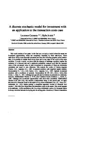
4.1. Effects of shocks to government spending instruments Figures 1-5 show the dynamic effects of transitory, but persistent shocks to government purchases of goods and services, government investment, public sector wage rates, government transfers and public sector employment. The magnitude of the shocks to government purchases of goods and services, government investment and government transfers is set in order to have a decrease in the various components of public spending at time t = 0 equal to 1% of steady-state output. The shock in public wage rates is set in order to have a decrease in the total public wage bill equal to 1% of steady-state output. Similarly, we choose the shock in public sector employment in order to achieve a decrease in the total public wage bill equal to 1% of initial output. The series plotted are percentage deviations from the steady-state, except for the net private foreign assets, the trade balance as share of GDP, the current account balance as share of GDP and the primary balance as share of GDP, which are percentage point changes.

35

4.1.1. Effects of shocks to government purchases of goods and services Figure 1 depicts the dynamic responses of some major macroeconomic variables to a persistent government shock in government purchases of goods and services equal to a 1% decrease in steady-state output. The first order effect is a positive wealth effect that leads optimizing households to increase current consumption and leisure (or to decrease labour supply in the private sector). 8 In contrast, liquidity constraint households reduce their consumption demand since they suffer income loss from the fall in hours worked, even though real wages increase due to the fall in private employment. The net effect on total private consumption is negative on impact, due to the presence of liquidity constraint households and real rigidities in the labour market (see e.g. Gali et al. (2007) for a discussion). In addition, the open economy set-up allows optimizing households to smooth consumption more effectively than when the economy is closed, by reducing the holdings of foreign assets, thereby dampening the response of private consumption in the short run. Nevertheless, the fall in total consumption is short-lived (only for one quarter), and its dynamic response in the following years of transition is denominated by the behaviour of optimizing households. The private sector real wage rate increases on impact, while the real return to capital decreases in order for the goods market to clear. The decrease in aggregate demand, coming from the initial reduction in public consumption, along with the decline in the inputs of production, leads to a fall in output both on impact and along the transition to the initial equilibrium. The estimated impact multiplier is found to be 0.96. 9 It is interesting to note that the fiscal contraction results to a rise in the debt-to-output ratio in the first quarters, due to the adverse effects on output. Regarding the variables related to the external sector, there is an increase in the real exchange rate in the short run, that is, a real depreciation. The reason is the violation of the uncovered interest parity, which must be restored by a rise in the real exchange rate relative to its expected future value. In turn, the increase in competitiveness results to a rise in exports in the short run, while there is a decrease in imports that is driven by the reduction in imported intermediate inputs. Consequently, there is an improvement in the trade balance and the current account balance as shares of GDP in the early years of transition. For instance, the trade balance 8

Optimizing households feel wealthier because the fiscal contraction increases the social resources that are available to the private sector, raising their permanent income. 9 The output multiplier on impact period after a change in government spending or tax policy instruments is defined as: ϕ t = ∆Yt / ∆X t , where ∆Yt and ∆X t are respectively level changes in output and the fiscal variable of interest relative to their pre-policy reform values.

36

and the current account balance as shares of GDP increase by around 0.13 and 0.11 percentage points on impact, in line with the results obtained in Erceg et al. (2005) for the U.S. economy.

Figure 1: Dynamic responses to a government purchases shock Total Private Consumption

40

10

0 20 Quarter

30

40

0.1 0 -0.1 0

20 Quarter

30

20

40

% Deviation 30

40

Trade Balance / GDP 0.1 0.05 0 20

40

60 80 Quarter

100

% Point Deviation

% Deviation % Point Deviation

0 20 Quarter

10

20 Quarter

40

30

60 80 Quarter

40

20 Quarter

-2 0

10

20 Quarter

30

0.1

0 40

60 80 Quarter

100

40

10

20 Quarter

20

40

60 80 Quarter

100

0 -0.5 -1 0

10

20 Quarter

30

40

0.6 0.4 0.2 0 40

60 80 Quarter

40

0.2 0.1 0

0

10

20 Quarter

30

40

30

40

0.5 0 -0.5 0

100

10

20 Quarter

Private Foreign Assets 0 -0.5 -1 0

Primary Balance / GDP

20

30

Imports

0.15 0.1 0.05 0 -0.05

40

0.05

30

Imported Intermediate inputs

Current Account Balance / GDP

20

0 -1 0

Real Wages - Private Sector

0

100

0 10

40

Exports

0.2

-0.2 0

30

-1

Imported consumption goods

0.2

10

20 Quarter

0.1 0.05 0

Domestic consumption goods

-0.2 0

10

% Deviation

0 -0.2 10

0

Real Exchange Rate % Deviation

% Deviation

Real Return to Private Capital

-0.4 0

0

1

Hours Worked-Private Sector

% Deviation

10

0.2

40

% Deviation

0.5

-0.5 0

30

Private Investment % Deviation

% Deviation

Private Capital Services

20 Quarter

% Deviation

0 -0.2 0

% Deviation

30

% Deviation

20 Quarter

10

20 Quarter

30

40

Total Public Debt / GDP % Deviation

10

% Point Deviation

-1 0

Consumption - Credit Constraint

0.4

% Point Deviation

-0.5

Consumption - Optimizing

0.2

% Deviation

% Deviation

% Deviation

Real Output 0

0.5 0 -0.5 -1 20

40

60 80 Quarter

100

Notes: (i) The series plotted are percentage deviations from the steady-state, except for the net private foreign assets, the trade balance as share of GDP, the current account balance as share of GDP and the primary balance as share of GDP, which are percentage point changes, (ii) a positive change in the trade balance, the current account balance and the primary balance as shares of GDP means an improvement in these variables.

4.1.2. Effects of shocks to government investment Figure 2 shows selected dynamic responses to a persistent government shock in public investment equal to a 1% decrease in steady-state output. The reduction in public investment implies a decrease in governmental absorption of recourses, as in the case of a decrease in public consumption, but now there are also supply-side effects, as a lower stock of public infrastructure leads to lower marginal products of private inputs. As a result, while private consumption and investment of optimizing households rise on impact, they both fall in the later years. At the same time, the reduction in hours worked and real wages induces liquidity constraint households to decrease consumption demand. Output is below its initial level all the time, while the contraction of output produces a rise in the debt-to-GDP ratio in the short run. The impact multiplier for output is estimated at 0.89. Finally, it should be noted that the reduction in public investment causes an increase in the real exchange rate that shifts foreign and domestic demand towards domestic goods,

37

particularly in the short run, and gives rise to an expansion in exports and a decrease in the value of imports. Consequently, the trade balance-to-output ratio increases by around 0.2 percentage points on impact, while the effect on the current account balance is also positive along the dynamic path.

Figure 2: Dynamic responses to a government investment shock Total Private Consumption

0 -0.5 50

100 Quarter

150

200

100 Quarter

% Deviation 150

0.2 0.1 0

20

40 60 Quarter

80

200

% Point Deviation

% Deviation % Point Deviation

0

100 Quarter

% Deviation 20

150

50

0

50

100 Quarter

150

200

Current Account Balance / GDP 0.15 0.1 0.05 50

100 Quarter

80

100 Quarter

150

150

0 -0.5 -1 0

0.2 0 -0.2 0

50

100

50 Quarter

0.8 0.6 0.4 0.2 0 40 60 Quarter

100 Quarter

150

200

150

200

0 -0.2 -0.4 0

80

50

100 Quarter

Private Foreign Assets 2 0 -2 0

Primary Balance / GDP

20

100

Imports

Imported Intermediate inputs

-0.05 -0.1 0

40 60 Quarter

50 Quarter

Real Wages - Private Sector

0.6 0.4 0.2 0

Imported consumption goods

-0.1 50

100 Quarter

-1 0

200

Exports

0 50

150

0 -0.2 -0.4 -0.6

200

0.2

150

Trade Balance / GDP

150

0.4

Domestic consumption goods

-0.2 0

100 Quarter

% Deviation

-0.1

50

100 Quarter

-0.5

Hours Worked-Private Sector

0 -1 0

50

Real Exchange Rate % Deviation

% Deviation

0

50

200

1

Real Return to Private Capital

-0.2

150

% Deviation

-1 0

100 Quarter

Private Investment % Deviation

% Deviation

Private Capital Services

50

% Deviation

200

0 -0.2 0

0

% Point Deviation

150

% Deviation

100 Quarter

% Deviation

50

-0.1 -0.15 0

% Point Deviation

-1 0

0.2

50

100 Quarter

150

200

Total Public Debt / GDP % Deviation

-0.5

Consumption - Credit Constraint

Consumption - Optimizing

-0.05

% Deviation

% Deviation

% Deviation

Real Output 0

0 -1 -2 20

40 60 Quarter

80

Notes: (i) The series plotted are percentage deviations from the steady-state, except for the net private foreign assets, the trade balance as share of GDP, the current account balance as share of GDP and the primary balance as share of GDP, which are percentage point changes, (ii) a positive change in the trade balance, the current account balance and the primary balance as shares of GDP means an improvement in these variables.

4.1.3. Effects of shocks to public sector wages Figure 3 summarizes the dynamic responses to a shock in the average wage rate of the public sector. Recall that the shock in the average wage rate is set in order to have a decrease in the total public wage bill equal to 1% of initial output. Cutting public sector wages reduces the disposable income of liquidity constraint households, leading to a reduction in consumption purchases. Regarding the behavior of optimizing households, the decrease in aggregate demand, driven by the lower consumption demand of liquidity constraint households, leads to a fall in the real return to private capital and generates an inter-temporal substitution effect that induces them to increase current consumption and leisure (or decrease labour supply in the private sector). In turn, the fall in labour supply produces a small, albeit negligible increase in private sector wages on impact. However, private sector wages fall in the following years of transition and converge

38

to the initial equilibrium from below. The negative response of both hours of worked and capital services, combined with the reduction in imported intermediate inputs, translate into a fall in output along the dynamic path to the initial steady state. Nevertheless, the negative impact on output is much smaller than in the case of a fiscal contraction in the form of lower government purchases on goods and services or public infrastructures. For instance, the output multiplier on impact period is estimated at 0.18. However, it should be stressed that the value of the multiplier depends on the share of liquidity constrained households. For instance, for a share of liquidity constraint households equal to 0.6, the impact multiplier is about 0.28. The debt ratio decreases on impact and converges to the initial equilibrium from below. Thus, in terms of output losses, reductions in public wages is a more desirable option for reducing public debt than cuts in public consumption and investment. Concerning the variables associated with the external sector, there is an increase in the real exchange that triggers a rise in exports. At the same time, the decrease in imports, driven mainly by the reduction in imported consumption goods, gives rise to an improvement in the trade and current account balance ratios. Figure 3: Dynamic responses to a public sector wage rate shock

0 -2 10 -3

-3

-0.5 -1 -1.5 -2 -2.5 4

6 8 10 Quarter

12

2

% Point Deviation

% Deviation x 10 Trade Balance / GDP

8 6 4 2 4

6 8 10 Quarter

12

2

14

-0.04 2

14

4

6 8 10 Quarter

12

0

-3

8 6 4 2 2

4

6 8 10 Quarter

12

4

6 8 10 Quarter

12

14

x 10 Imported Intermediate inputs

-5 -15 2

x 10 Current Account Balance / GDP

14

4

6 8 10 Quarter

12

14

6 8 10 Quarter

50

0 -0.02 -0.03

12

2

4

6 8 10 Quarter

12

14

Private Foreign Assets -0.01 -0.02 -0.03 10

20

30 40 Quarter

50

Total Public Debt / GDP

0.06 0.04 0.02 0 4

30 40 Quarter

-0.01

Primary Balance / GDP

2

20

Imports

-10

14

10

14

-3

0

14

-3

2

12

12

1 0 -1 -2

Exports

x 10

-0.02

% Point Deviation

% Deviation

-0.04 12

6 8 10 Quarter

6 8 10 Quarter

14 12 10 8 6 4

Imported consumption goods

0

6 8 10 Quarter

4

4 -3

5

14

-0.02 4

2

50

10

Domestic consumption goods

2

30 40 Quarter

% Deviation

2

20

0 -5 -10 -15

Real Exchange Rate % Deviation

x 10

% Deviation

% Deviation

x 10 Real Return to Private Capital

2 4 6 8 10 12 14 Quarter -4 x 10 Real Wages - Private Sector

% Deviation

2

14

0 -0.05 -0.1 -0.15

10 20 30 40 50 Quarter -3 x 10 Hours Worked-Private Sector

14

% Point Deviation

12

12

% Deviation

-10

6 8 10 Quarter

0 -5

Private Investment % Deviation

0

6 8 10 Quarter

4 -3

5

% Deviation

2 x 10

Consumption - Credit Constraint % Deviation

-0.04

14

-5

4

% Deviation

-0.02

% Deviation

% Deviation

2 4 6 8 10 12 Quarter -3 x 10 Private Capital Services

2

-4 x 10 Consumption - Optimizing

Total Private Consumption 0

% Point Deviation

Real Output

x 10

% Deviation

% Deviation

-3

0 -5 -10 -15

14

0 -0.02 -0.04 10

20

30 40 Quarter

50

Notes: (i) The series plotted are percentage deviations from the steady-state, except for the net private foreign assets, the trade balance as share of GDP, the current account balance as share of GDP and the primary balance as share of GDP, which are percentage point changes, (ii) a positive change in the trade balance, the current account balance and the primary balance as shares of GDP means an improvement in these variables.

39

4.1.4. Effects of shocks to government transfers Figure 4 shows selected dynamic responses to a shock in public transfers equal to a 1% decrease in steady-state output. The reduction in government transfers induces a decrease in total consumption driven by the fall in the consumption demand of liquidity constraint households, who experience a loss in their disposable income. At the same time, optimizing households decrease both their labour and capital supply, while they also reduce the holdings of foreign assets in an attempt to smooth consumption over time. Since employment and capital services fall, output also falls. In addition, the reduction in domestic interest rates leads to a real depreciation, that is, an increase in competitiveness that gives rise to an expansion in real exports. The reduction in consumption purchases dampens imports, particularly the level of imported consumption goods, and hence produces an improvement in the trade balance and the current account balance as shares of GDP. Finally, the debt-to-output ratio decrease both on impact and during the transition to the initial equilibrium.

Figure 4: Dynamic responses to a government transfer shock

10 Quarter

0.04 0.02 5

% Deviation

-0.2

% Point Deviation

5

10 Quarter

Trade Balance / GDP

0.02 5

10 Quarter

15

10 Quarter

0

-0.2 5

10 Quarter

15

Current Account Balance / GDP 0.04 0.02 5

10 Quarter

15

10 Quarter

-3 -4

% Deviation

15

5

Exports

5

10 Quarter

5

10 Quarter

15

5

10 Quarter

15

10 Quarter

15

Private Foreign Assets 0 -0.2 -0.4 5

Primary Balance / GDP 0.8 0.6 0.4 0.2 0 5

15

0 -0.05 -0.1 -0.15

15

Imported Intermediate inputs 0 -0.02 -0.04 -0.06 -0.08

10 Quarter

Imports

0.08 0.06 0.04

15

-0.1

15

0.04

5

Imported consumption goods

% Point Deviation

% Deviation

Domestic consumption goods 0

30

0.06

15 10 5 Quarter -3 x 10 Real Wages - Private Sector

30

0 -0.02 -0.04 -0.06

Real Exchange Rate

15

-0.1

20 Quarter

20 Quarter

% Deviation

-10

10

10

10 Quarter

15

Total Public Debt / GDP % Deviation

0 -5

5

0 -0.01 -0.02

15

-3 x 10 Real Return to Private Capital

% Deviation

% Deviation 10 Quarter

-5 -10

Hours Worked-Private Sector

% Deviation

% Deviation

5

15

Private Investment

% Deviation

% Deviation

Private Capital Services

10 Quarter

Consumption - Credit Constraint 0 -0.2 -0.4 -0.6 -0.8

% Deviation

5

0

% Point Deviation

-0.2

15

0 -0.02 -0.04 -0.06

% Deviation

-0.1

% Deviation

10 Quarter

0

% Point Deviation

5

-3 x 10 Consumption - Optimizing

Total Private Consumption % Deviation

% Deviation

Real Output 0 -0.02 -0.04 -0.06 -0.08

-0.2 -0.4 -0.6

10

20 Quarter

30

Notes: (i) The series plotted are percentage deviations from the steady-state, except for the net private foreign assets, the trade balance as share of GDP, the current account balance as share of GDP and the primary balance as share of GDP, which are percentage point changes, (ii) a positive change in the trade balance, the current account balance and the primary balance as shares of GDP means an improvement in these variables.

40

4.1.5. Effects of shocks to public employment Figure 5 illustrates the dynamic effects of a shock in public sector employment. The shock is set in order to achieve a decrease in the total public wage bill equal to 1% of steady state output. The decrease in public employment lowers the labour income of the liquidity constraint households, inducing a sizable reduction in consumption demand. At the same time, the decrease in public employment leads optimizing households to increase labour supply in the private sector, as well as consumption purchases. This behavior is explained by the leisureconsumption intra-temporal condition, which given the fall in total employment, it requires an increase in hours worked (and thus a decrease in the private wage rate) or consumption. Eventually, both labour supply and consumption increases, while the real wage rate in the private sector falls. The net effect on total private consumption is, however, negative. Despite the rise in hours worked, output decreases on impact due to the fall in private capital services and imported intermediate inputs in the short run. However, there is an expansion of output in the following years of transition, triggered by the rise in the inputs of production. At the same time, the public debt-to-output ratio decreases significantly both on impact and along the dynamic path to the initial equilibrium. Thus, in terms of output losses, a reduction in public employment seems to be the most desirable policy in improving public finances. Finally, note that the reduction in public employment induces a real depreciation in the early years of transition that boosts real exports and hence leads to an improvement in the trade balance and the current account balance ratios. For instance, the trade balance and the current account balance as shares of GDP increase by around 0.19 percentage points on impact.

41

Figure 5: Dynamic responses to a public sector employment shock

60 80 Quarter

20

100

0.1 0.05 0 -0.05

20

40

60 80 Quarter

0 20

% Point Deviation

% Deviation 20

40

60 80 Quarter

0.15 0.1 0.05 0 20

40

60 80 Quarter

100

60 80 Quarter

40

0

-0.4 20

40

60 80 Quarter

20

60 80 Quarter

40

60 80 Quarter

20

100

40

60 80 Quarter

20

20

100

100

1 0.5 0 40

60 80 Quarter

50

40

60 80 Quarter

100

0 -0.1 -0.2

100

40

60 80 Quarter

100

Private Foreign Assets 0 -1 -2 20

Primary Balance / GDP

20

30 40 Quarter

Imports

0.1 0.05 0 -0.05

100

0.15 0.1 0.05 0 40

20

0 -0.05 -0.1 -0.15

100

Imported Intermediate inputs

Current Account Balance / GDP

20

60 80 Quarter

0.6 0.4 0.2 0

100

-0.2

100

Trade Balance / GDP

40

10

Real Wages - Private Sector

Exports

Imported consumption goods

% Point Deviation

% Deviation

-0.4

0 20

0.2

Domestic consumption goods

-0.2

0.1

100

0.4

100

0

60 80 Quarter

-2

50

0.2

Real Exchange Rate % Deviation

% Deviation

Real Return to Private Capital

40

30 40 Quarter

% Deviation

40

0.6 0.4 0.2 0

% Deviation

20

20

0 -1

Hours Worked-Private Sector

% Deviation

-0.1

10

100

% Deviation

% Deviation

% Deviation

0

60 80 Quarter

Private Investment

Private Capital Services 0.1

40

0.2

% Deviation

20

50

% Deviation

-0.4

Consumption - Credit Constraint

0.4

40

60 80 Quarter

100

Total Public Debt / GDP % Deviation

30 40 Quarter

-0.2

% Point Deviation

20

0

% Point Deviation

% Deviation

% Deviation

10

Consumption - Optimizing % Deviation

Total Private Consumption

Real Output 0.15 0.1 0.05 0 -0.05

-1 -2 -3 20

40

60 80 Quarter

100

Notes: (i) The series plotted are percentage deviations from the steady-state, except for the net private foreign assets, the trade balance as share of GDP, the current account balance as share of GDP and the primary balance as share of GDP, which are percentage point changes, (ii) a positive change in the trade balance, the current account balance and the primary balance as shares of GDP means an improvement in these variables.

4.2. Effects of shocks to tax policy instruments Figures 6-8 show the dynamic effects of transitory, but persistent shocks to the tax rates on consumption, labour income and capital income. The shocks to different tax instruments are set so that to achieve an increase in the different categories of tax revenues by 1% of initial output. The series plotted are percentage deviations from the steady-state, except for the net private foreign assets, the trade balance as share of GDP, the current account balance as share of GDP and the primary balance as share of GDP, which are percentage point changes.

4.2.1. Effects of shocks to the labour tax rate Figure 6 depicts the dynamic responses to a persistent shock in the tax rate on labour income. The increase in the labour income tax rate causes a negative wealth effect that induces optimizing households to reduce current consumption and leisure (and thus increase current labour supply). But, at the same time, the higher tax rate reduces the net return to labour inducing an intra-temporal substitution effect that leads households to reduce current labour supply and consumption. As the impulses show, the latter substitution effect dominates, so that labour supply and hours of work fall. Eventually, output decreases and so does private

42

consumption. The impact multiplier for output is estimated at -1.24. At the same time, the decrease in the after-tax labour income forces liquidity constraint households to reduce consumption demand. It is worth noting that the debt-to-output ratio increases during the early years transition (for more than 10 quarters), which reflects the fact that a fiscal consolidation aiming at reducing public debt via increases in labour taxes is not a good idea (see also Forni et al. (2011) and Papageorgiou (2012)). Regarding the impact of the higher labour tax rate on the variables related to the external sector, we observe a decrease in the real exchange rate in the short run, that is, a real appreciation. The loss in competitiveness causes a sizable reduction in the demand for exports and hence a deterioration in the trade balance in the short run. Nevertheless, the significant fall in imports in the latter years causes an improvement in the trade balance.

Figure 6: Dynamic responses to a shock in the tax rate on labour income

10

20 Quarter

10

30

10

20 Quarter

10

30

% Point Deviation

% Deviation 10

20 Quarter

0.01 0 -0.01 10

20 Quarter

30

20 Quarter

-0.1 -0.15 10

20 Quarter

20 Quarter

30

% Deviation

0 10

0 -0.05 -0.1 20 Quarter

-0.1 -0.15 10

30

0.1 0.05 0 20 Quarter

30

20 Quarter

30

Private Foreign Assets 0 -0.05 10

Primary Balance / GDP

10

30

-0.05

30

Imported Intermediate inputs

10

20 Quarter

Imports

-0.2 20 Quarter

30

0.1

30

-0.1 10

20 Quarter

0.05

Exports

-3 x 10 Current Account Balance / GDP

10

20 Quarter

0

30

5 0 -5 -10 -15

10

Real Wages - Private Sector % Deviation

10

30

-0.05

30

Trade Balance / GDP

-0.2

Imported consumption goods

% Point Deviation

% Deviation

Domestic consumption goods -0.05 -0.1 -0.15

0 -0.1

30

0 -0.05 -0.1 -0.15

-0.4

Hours Worked-Private Sector

Real Exchange Rate % Deviation

% Deviation

Real Return to Private Capital 0 -0.05 -0.1 -0.15

20 Quarter

-0.2

30

% Deviation

-0.02

0 -0.05 -0.1 -0.15

20 Quarter

20 Quarter

30

Total Public Debt / GDP % Deviation

0

10

30

% Deviation

0.02

-0.1

Private Investment % Deviation

% Deviation

Private Capital Services

20 Quarter

Consumption - Credit Constraint

% Point Deviation

10

30

-0.05

% Deviation

20 Quarter

-0.1 -0.15

% Deviation

10

-0.05

% Point Deviation

-0.1 -0.15

Consumption - Optimizing % Deviation

Total Private Consumption % Deviation

% Deviation

Real Output 0 -0.05

0.1 0.05 0 10

20 Quarter

30

Notes: (i) The series plotted are percentage deviations from the steady-state, except for the net private foreign assets, the trade balance as share of GDP, the current account balance as share of GDP and the primary balance as share of GDP, which are percentage point changes, (ii) a positive change in the trade balance, the current account balance and the primary balance as shares of GDP means an improvement in these variables.

43

4.2.2. Effects of shocks to the consumption tax rate Figure 7 illustrates the dynamic responses to a persistent shock in the tax rate on consumption. There is again a negative wealth effect that pushes optimizing households to decrease current consumption and leisure (and thus increase labour supply). At the same time, the higher consumption tax rate induces an intra-temporal substitution effect that leads optimizing households to reduce labour supply and consumption. As the impulses show, the latter substitution effect dominates the former wealth effect, so that labour supply and hours of work fall, together with private consumption. The consumption demand of liquidity constraint households also falls due to the decrease in the disposable income. Consequently, output also falls, while the impact multiplier for output is estimated at -0.49, which is much lower than in the case of an increase in labour taxes. In contrast to the case of a rise in labour taxes, the increase in the consumption tax rate induces an increase in the real exchange rate, that is, a real depreciation that boosts exports. The rise in exports, in combination with the fall in imports, causes an improvement in the trade balance and the current account balance.

Figure 7: Dynamic responses to a shock in the tax rate on consumption

5

10 Quarter

5

% Deviation x 10 Trade Balance / GDP

12 10 8 6 4 2 5

10 Quarter

15

15

0 -0.02 -0.04 -0.06 5

15

-3

10 Quarter

14 12 10 8 6 4

10 Quarter

5

10 Quarter

15

5

10 Quarter

% Deviation x 10

10 Quarter

0

-0.03 10 Quarter

0 -0.02 -0.04 5

15

-0.02 5

15

10 Quarter

15

10 Quarter

15

Private Foreign Assets 0 -0.02 -0.04 10

Primary Balance / GDP 0.08 0.06 0.04 0.02 0 5

15

Imports

-0.01

x 10 Current Account Balance / GDP 10 8 6 4 2

15

Imported Intermediate inputs

15

-3

10 Quarter

6 4 2 0

Exports

5

Imported consumption goods

% Point Deviation

% Deviation

% Point Deviation

10 Quarter

-3

5

Domestic consumption goods

5

5

50

10

15

0 -0.02 -0.04 -0.06

30 40 Quarter

% Deviation

% Deviation

% Deviation

x 10

-2 -4 -6 -8 -10 -12

20

Real Exchange Rate

% Deviation

10 -3

5 10 15 Quarter -3 x 10 Real Wages - Private Sector

15

% Point Deviation

15

x 10 Real Return to Private Capital

10 Quarter

0 -0.01 -0.02 -0.03

% Deviation

10 Quarter

-3

Consumption - Credit Constraint 0 -0.05 -0.1 -0.15

Hours Worked-Private Sector

% Point Deviation

5

6 4 2 0 -2

5

15

Private Investment

x 10

% Deviation

0 -5 -10 -15

10 Quarter

-0.01 -0.02 -0.03 -0.04 -0.05

20

30 40 Quarter

50

Total Public Debt / GDP % Deviation

5 -3

% Deviation

% Deviation

5 10 15 Quarter -3 x 10 Private Capital Services

Consumption - Optimizing % Deviation

0 -0.02 -0.04 -0.06

% Deviation

Total Private Consumption % Deviation

% Deviation

Real Output 0 -0.01 -0.02 -0.03

0 -0.02 -0.04 10

20

30 40 Quarter

50

Notes: (i) The series plotted are percentage deviations from the steady-state, except for the net private foreign assets, the trade balance as share of GDP, the current account balance as share of GDP and the primary balance as share of GDP, which are percentage point changes, (ii) a positive change in the trade balance, the current account balance and the primary balance as shares of GDP means an improvement in these variables.

44

4.2.3. Effects of shocks to the capital income tax rate Figure 8 summarizes the dynamic responses to a persistent shock in the tax rate on capital income. An increase in the capital income tax rate has a negative wealth effect that pushes optimizing households to decrease current consumption and leisure (and thus increase labour supply). At the same time, the fall in the net return to capital, which reduces private investment and capital over time, produces an inter-temporal substitution effect that leads households to increase current consumption and leisure. As can be seen from Figure 8, the net effect on consumption and leisure is negative so that hours of work rise and consumption falls in the short run. Despite the rise in hours worked, output falls during the transition due to the sizable reduction in capital services. The impact multiplier is estimated at 0.73. The increase in labour supply reduces the real wage rate, leading to a reduction in the labour of the liquidity constraint households who are forced to reduce consumption demand. The fall in aggregate consumption dampens imports, while at the same time the reduction in the real exchange rate triggers a reduction in exports and hence gives rise to a deterioration in the trade balance in the short run. Finally, it is interesting to point out that, as in the case of higher labour taxes, the debt-to-output rises in the short run due to the contractionary effects that capital taxes have on output.

Figure 8: Dynamic responses to a shock in the tax rate on capital income

20 Quarter

10

0.1 0.08 0.06 0.04 0.02 10

20 Quarter

0

-0.04 10

30

% Point Deviation

% Deviation 10

20 Quarter

2 0 -2 -4 -6 -8

10

20 Quarter

30

20 Quarter

10

2 0 -2 -4 -6 -8

20 Quarter

20 Quarter

0 -0.02 -0.04 -0.06

% Deviation 10

20 Quarter

10

20 Quarter

30

30

-0.005 -0.01 -0.015 -0.02 -0.025

0.04 0.02 0 20 Quarter

30

30

10

20 Quarter

30

Private Foreign Assets 0 -0.02 -0.04 10

Primary Balance / GDP

10

20 Quarter

Imports

-0.005 -0.01 -0.015 -0.02 -0.025 10

30

-0.04

30

Imported Intermediate inputs

30

30

20 Quarter

20 Quarter

-0.02

Exports

-3 x 10 Current Account Balance / GDP

10

10

Real Wages - Private Sector % Deviation

0 10

30

-0.005 -0.01 -0.015 -0.02

30

-3 x 10 Trade Balance / GDP

10

Imported consumption goods

% Point Deviation

% Deviation

Domestic consumption goods -0.005 -0.01 -0.015 -0.02 -0.025

20

30

-0.02

-0.02

x 10 Hours Worked-Private Sector

Real Exchange Rate % Deviation

% Deviation

Real Return to Private Capital

20 Quarter

-0.01

-3

-0.02 -0.04 -0.06 -0.08

30

0

30

% Deviation

10

20 Quarter

20 Quarter

30

Total Public Debt / GDP % Deviation

-0.02 -0.04 -0.06 -0.08 -0.1 -0.12

10

30

Private Investment % Deviation

% Deviation

Private Capital Services

20 Quarter

% Point Deviation

10

30

% Deviation

20 Quarter

Consumption - Credit Constraint

-0.005 -0.01 -0.015 -0.02

% Deviation

10

% Deviation

-0.03

-0.005 -0.01 -0.015 -0.02

% Point Deviation

-0.02

Consumption - Optimizing % Deviation

Total Private Consumption % Deviation

% Deviation

Real Output -0.01

0.01 0 -0.01 -0.02 20

40 Quarter

60

Notes: (i) The series plotted are percentage deviations from the steady-state, except for the net private foreign assets, the trade balance as share of GDP, the current account balance as share of GDP and the primary balance as share of GDP, which are percentage point changes, (ii) a positive change in the trade balance, the current account balance and the primary balance as shares of GDP means an improvement in these variables.

45

4.3. Effects of shocks to total factor productivity and world output Figures 9 and 10 depict the dynamic responses to a temporary unitary increase in the innovations of total factor productivity and world output, respectively. The shock in total factor productivity generates a positive wealth effect that leads optimizing households to increase current consumption and leisure. At the same time, the increase in the marginal productivity of private inputs gives households the incentive to substitute away from leisure and increase consumption. As Figure 9 shows, optimizing households decrease current labour supply, whereas they increase consumption and investment demand. The fall in hours of work triggers a rise in real private sector wages and hence on the disposable income of liquidity constraint households, who in turn, increase consumption purchases. The real interest rate rises in order to restrain the increase in domestic demand and triggers a depreciation of the real exchange rate. In turn, the real depreciation gives rise to an expansion in exports and an improvement in the trade balance, although imports of both consumption goods and intermediate inputs increase. Despite the fall in hours worked and capital services in the short run, the positive technology shock, combined with the higher imported inputs, generate an expansion in output along the dynamic path.

Figure 9: Dynamic responses to a shock in total factor productivity

10

20 Quarter

0.6 0.4 0.2 0 10

30

0.8 0.6 0.4 0.2 0 10

20 Quarter

1

0 10

30

% Deviation

0.5 0.4 0.3 0.2 0.1

% Point Deviation

10

20 Quarter

0.2 0.1 0 10

20 Quarter

30

% Deviation

-0.4 10

0.2 10

20 Quarter

0.2 0.1 0 10

20 Quarter

30

20 Quarter

10

1

0.8 0.6 0.4 0.2 10

0.4 0.2 10

20 Quarter

30

0.15 0.1 0.05 0 20 Quarter

30

0.2 10

30

20 Quarter

30

Private Foreign Assets 0.05 0 -0.05 -0.1 -0.15 20

Primary Balance / GDP

10

20 Quarter

0.4

30

Imported Intermediate inputs

0

30

Imports

0.5 0 20 Quarter

20 Quarter

Real Wages - Private Sector

30

1.5

10

30

Current Account Balance / GDP

0.1

Exports

30

0.4

30

Trade Balance / GDP

0

Imported consumption goods

% Point Deviation

% Deviation

Domestic consumption goods

20 Quarter

0.2

30

-0.2

30

0.5

0.3

Hours Worked-Private Sector

Real Exchange Rate % Deviation

% Deviation

Real Return to Private Capital

20 Quarter

20 Quarter

% Deviation

-0.4

10

30

% Deviation

0 -0.2

0.2

Private Investment % Deviation

% Deviation

Private Capital Services

20 Quarter

Consumption - Credit Constraint

% Point Deviation

10

30

0.4

40 60 80 100 120 140 Quarter

Total Public Debt / GDP % Deviation

20 Quarter

% Deviation

10

% Deviation

0

% Deviation

0.2

0.3 0.2 0.1

% Point Deviation

0.4

Consumption - Optimizing % Deviation

Total Private Consumption % Deviation

% Deviation

Real Output 0.6

-0.2 -0.4 -0.6 -0.8 20

40 60 80 100 120 140 Quarter

Notes: (i) The series plotted are percentage deviations from the steady-state, except for the net private foreign assets, the trade balance as share of GDP, the current account balance as share of GDP and the primary balance as share of GDP, which are percentage point changes, (ii) a positive change in the trade balance, the current account balance and the primary balance as shares of GDP means an improvement in these variables.

46

Figure 10 shows the effects from a rise in world output by 1%. The first order effect is an increase in the demand for exports that induces an expansion in domestic output and a real exchange appreciation. The higher output allows both types of households to increase consumption purchases, whereas the real exchange appreciation shifts the consumption demand towards imported consumption goods. Eventually, there is an improvement in the trade balance and the current account balance ratios in the short run.

Figure 10: Dynamic responses to a shock in world output

20 40 60 80 100 120 140 Quarter

% Deviation

% Deviation

0 20 40 60 80 100 120 140 Quarter

% Point Deviation

% Point Deviation

0.05

Current Account Balance / GDP 0.1 0.05 0 20 40 60 80 100 120 140 Quarter

% Deviation % Deviation

Imports % Deviation

0.6 0.4 0.2 0

0.06 0.04 0.02 20 40 60 80 100 120 140 Quarter

20 40 60 80 100 120 140 Quarter

Imported Intermediate inputs 0.08 0.06 0.04 0.02 0

20 40 60 80 100 120 140 Quarter

20 40 60 80 100 120 140 Quarter 0.1

% Deviation

0.04

20 40 60 80 100 120 140 Quarter

Exports

Imported consumption goods 0.06

0.03 0.025 0.02

20 40 60 80 100 120 140 Quarter

20 40 60 80 100 120 140 Quarter

Domestic consumption goods

Trade Balance / GDP

% Deviation

-0.05 -0.1 -0.15 -0.2 -0.25

20 40 60 80 100 120 140 Quarter

0.02 0.01 0

20 40 60 80 100 120 140 Quarter

Real Wages - Private Sector

20 40 60 80 100 120 140 Quarter

Private Foreign Assets 0.4 0.2 0

-3

x 10 Primary Balance / GDP 20 10 0 20 40 60 80 100 120 140 Quarter

20 40 60 80 100 120 140 Quarter

Total Public Debt / GDP % Deviation

0.03 0.02 0.01 0 -0.01

0.06 0.04 0.02 0 -0.02

Real Exchange Rate % Deviation

% Deviation

Real Return to Private Capital

20 40 60 80 100 120 140 Quarter

Hours Worked-Private Sector

% Deviation

0

0.06 0.04 0.02 0 -0.02 -0.04

Consumption - Credit Constraint 0.12 0.1 0.08 0.06 0.04 0.02

20 40 60 80 100 120 140 Quarter

Private Investment % Deviation

% Deviation

0.04 0.02

0.04

20 40 60 80 100 120 140 Quarter

Private Capital Services 0.06

0.06

% Point Deviation

20 40 60 80 100 120 140 Quarter

% Deviation

0

0.07 0.06 0.05 0.04 0.03

% Point Deviation

0.05

Consumption - Optimizing

Total Private Consumption % Deviation

% Deviation

Real Output 0.1

-0.05 -0.1 20 40 60 80 100 120 140 Quarter

5. Concluding remarks In this paper we have examined the dynamic properties of a DSGE model developed for quantitative policy analysis. The model was calibrated to the Greek economy at a quarterly frequency over the 2000q1-2011q4 period. Our approach in examining the dynamic properties of the model involved using impulse response functions to a number of shocks and analyzing the main transmission channels through which the shocks influence the macroeconomy. The results suggest that reductions in public spending are associated with improvements in fiscal and external imbalances. In terms of output losses, the most desirable way to reduce fiscal and external imbalances is through cuts in public sector wages, government transfers and public

47

sector employment. In contrast, the most harmful option for reducing fiscal and external imbalances seems to be an increase in labour income taxes. We acknowledge that the model assumes away a number of nominal frictions that have been found important in the data. Adding such features is an interesting extension. Estimating the model and examining its forecasting performance are also important future objectives.

References Adolfson, M., S. Laseen, J. Linde, Villani, M., 2007. Bayesian estimation of an open economy DSGE model with incomplete pass-through. Journal of International Economics, 72, 481-511. Angelopoulos Κ., Philippopoulos, A., Vassilatos, V., 2009. The social cost of rent seeking in Europe. European Journal of Political Economy, 25, 280-299. Ardagna, S., Caselli, F., Lane, T., 2004. Fiscal discipline and the cost of public debt service: Some estimates for OECD countries. NBER Working Paper No. 10788. Baier, S., Glomm, G., 2001. Long-run growth and welfare effects of public policies with distortionary taxation. Journal of Economic Dynamics and Control 25, 2007-2042. Baxter M. King, R., 1993. Fiscal policy in general equilibrium. American Economic Review. 83, 315-334. Blanchard, O., Gali, J., 2007. Real wage rigidities and the new Keynesian model. Journal of Money Credit and Banking 39, 35-66. Braun R., 1994. Tax disturbances and real economic activity in the post-war United States. Journal of Monetary Economics, 33, 441-462. Burnside, C., Eichenbaum, M., Fisher, J., 2004. Fiscal shocks and their consequences. Journal of Economic Theory 115, 89-117. Coenen, G., Straub, R.., Trabandt, M., 2012. Fiscal policy and the great recession in the euro area. American Economic Review, Papers and Proceedings, 102, 71-76. Coenen, G., Straub, R.., Trabandt, M., 2013. Gauging the effects of fiscal stimulus packages in the euro area. Journal of Economic Dynamics and Control, 32, 367-386. Cogan J., Cwik, T., Taylor, J., Wieland, V., 2010. New Keynesian versus old Keynesian government spending multipliers. Journal of Economic Dynamics and Control, 34, 281-285. Cooley, T., Prescott, E., 1995. Economic growth and fluctuations, in Frontiers of Business Cycle Research, edited by T. Cooley, Princeton University Press, Princeton. Chari V.V., Christiano, L., Kehoe, P., 1994. Optimal fiscal policy in a business cycle model. Journal of Political Economy, 102, 617-652.

48

Christiano L.J., Eichenbaum, M., 1992. Current real business cycle theories and aggregate labor market fluctuations. American Economic Review, 82, 430-450. Christiano, L.J., Eichenbaum, M., Evans, C., 2005. Nominal rigidities and the dynamic effects of a shock to monetary policy. Journal of Political Economy 113, 1-45. Christiano, L.J., Trabandt, M., Walentin, K., 2011. Introducing financial frictions into a small open economy model. Journal of Economic Dynamics and Control, 35, 1999-2041. Conesa, J.C., Kehoe, T., Ruhl, K., 2007. Modeling great depressions: the depreciation in Finland in the 1990s. Federal Reserve Bank of Minneapolis Quarterly Review 31, 16-44. Economides G., Philippopoulos, A., Vassilatos, V., 2011. Public providers versus private providers of public goods: A general equilibrium study of the role of the state. CESifo, Working Paper, no. 3487. Economides G., Papageorgiou, D., Philippopoulos, A., Vassilatos, V., 2012. Smaller Public Sectors in the Euro Area: Aggregate and Distributional Implications. CESifo Economic Studies, doi: 10.1093/cesifo/ifs041. Erceg, C., Guerrieri, L., Gust, C., 2005. Expansionary Fiscal Shocks and the US Trade Deficit. International Finance, 8, 363-397. European Commission, 2010. The economic adjustment programme for Greece. European Economy, Occasional Papers No. 61, May 2010. European Commission, 2012. Report in public finances in EMU - 2012. European Economy No. 4/2012. Forni, L., Monteforte, L., Sessa, L., 2009. The general equilibrium effects of fiscal policy: estimates for the euro area. Journal of Public Economics 93, 559-585. Forni, L., Gerali, A., Pisani, M., 2010. The macroeconomics of fiscal consolidations in euro area countries. Journal of Economic Dynamics and Control 34, 1791–1812. Gali J., Lopez-Salido, D., Valles, J., 2007. Understanding the effects of government spending on consumption. Journal of the European Economic Association, 5, 227-270. Gogos, S.G., Mylonidis, N., Papageorgiou, D., Vassilatos, V., 2012. Greece 1979-2001: A (First) Great Depression Seen From the Basic RBC Model Perspective, AUEB – Department of Economics, Working Paper Series, 01-2012. Jonsson G., Klein, P., 1996. Stochastic fiscal policy and the Swedish business cycle. Journal of Monetary Economics, 38, 245-268. Kehoe, T., Prescott, E., 2002. Great depressions of the twentieth century. Review of Economic Dynamics 5, 1-18. King R., Rebelo, S., 1999. Resuscitating real business cycles, in Handbook of Macroeconomics, volume 1B, edited by J. Taylor and M. Woodford, 927-1007, North-Holland, Amsterdam.

49

Klein, P., 2000. Using the generalized Schur form to solve a multivariate linear rational expectations model. Journal of Economic Dynamics and Control 24, 1405–1423. Kollintzas T., Vassilatos, V., 2000. A small open economy model with transaction costs in foreign capital, European Economic Review 44, 1515-1541. Kollintzas, T., Papageorgiou, D., Vassilatos V., 2012. An explanation of the Greek crisis: “the insiders – outsiders society”. CEPR Discussion Paper No. 8996. Kydland, F., 2006. Quantitative aggregate economics. American Economic Review, 96, 13731383. Lapatinas, 2009. Labour adjustment costs estimation of a dynamic discrete choice model using panel data for Greek manufacturing firms. Labour Economics, 16, 521-533. Malley J., Philippopoulos, A., Woitek, U., 2007. Electoral uncertainty, fiscal policy and macroeconomic fluctuations. Journal of Economic Dynamics and Control, 31, 1051-1080. Malley, J., Philippopoulos, A., Woitek, U., 2009. To react or not? Fiscal policy, volatility and welfare in the EU-3. European Economic Review 53, 689–714. McGrattan, E., 1994. The macroeconomic effects of distortionary taxation. Journal of Monetary Economics, 33, 573-601. McGrattan E., 2006. Real business cycles, Federal Reserve Bank of Minneapolis, Staff Report 370. Mendoza, E., Razin, A., Tesar, L., 1994. Effective tax rates in macroeconomics: cross-country estimates of tax rates on factor incomes and consumption. Journal of Monetary Economics 34, 297-323. Mertens, K., Ravn, M., 2011. Understanding the aggregate effects of anticipated and unanticipated policy shocks. Review of Economic Dynamics 14, 27–54. Molnár, M., Bottini, N., 2010. How Large Are Competitive Pressures in Services Markets? Estimation of Mark-ups for Selected OECD Countries. OECD Journal: Economic Studies. Papageorgiou, D., 2009. Macroeconomic Implications of Alternative Tax Regimes: The Case of Greece. Bank of Greece Working Paper No. 97. Papageorgiou, D., 2012. Fiscal policy reforms in general equilibrium: the case of Greece. Journal of Macroeconomics, 34, 504-522. Papageorgiou, D., Philippopoulos, A., Vassilatos, V. (2011). A toolkit for the study of fiscal policy in Greece, (2011), in Essays in Economics: Applied studies for the Greek economy, edited by S. Balfousias, P. Hatzipanayotou, C. Kanellopoulos, Centre of Planning and Economic Research (KEPE), 165-201. Ratto M., Roeger, W., in t’ Veld, J., 2009. QUEST III: An estimated open economy DSGE model of the euro area with fiscal and monetary policy. Economic Modeling, 26, 222-233.

50

Reinhart, C., Rogoff, K., 2009, This Time is Different, Princeton University Press. Rebelo, S., 2005. Real business cycle models: past, present and future. Scandinavian Journal of Economics, 107, 217-238. Rezitis, A., Kalantzi, M., 2011. Investigating Market Structure of the Greek Manufacturing Industry: A Hall-Roeger Approach. International Atlantic Economic Society, 39, 383-400. Schmitt-Grohé S. and Uribe M., 2003. Closing Small Open Economies. Journal of International Economics, 61, 163-185. Smets, F., Wouters, R., 2003. An estimated dynamic stochastic general equilibrium model of the euro area. Journal of the European Economic Association, 5, 1123-1175. Smets, F., Wouters., R., 2007. Shocks and frictions in US business cycle: a Bayesian DSGE approach. American Economic Review 97, 586-606. Uhlig, H., 2010. Some fiscal calculus. American Economic Review 100, 30-34.

Appendix: Stationary decentralized competitive equilibrium All variables (except of hours worked) grow at the constant growth rate γ z . We thus need to make them stationary. For any per capita variable X t define xt = X t / Z t . Also, define

λt = λt / Z t(1−γ

2

)(1−σ ) −1

, while note that qt does not grow since qt = µt / λt .

(

)

1−σ

 ci − ξ c / γ c i γ 1 (1 − h )γ 2 y g 1−γ 1 −γ 2  ( t )  z ) t −1 t 1  t ( λt = c γ 1 Pt (1 + τ tc ) cti − (ξ c / γ z ) cti−1 i c i c c γ 2 ct − (ξ / γ z ) ct −1 Pt (1 + τ t ) = wtp ≡ MRSt l 1 − ht 1−τt γ1

(1 − τ ) r k t

t

k

= qtδ ρφ utφ −1

γ z λt = β Et λt +1Rtb+1 γ k

p z t +1

(A2) (A3) (A4)

2  ξk γ i   z t = (1 − δ ut ) k + 1 −  − γ z   it 2  it −1   

ρ φ

(A1)

p t

(A5)

Rtb − Rt = Et (Qt +1 / Qt )

(A6)

λ γ z q=t β t+1 (1 − τ tk+1 )( rtk+1ut +1 ) + qt +1 (1 − δ ρ utφ+1 ) λt

(A7)

51 2  ξk γ i  γ i γ i  z t 1 = qt 1 −  −γz  −ξk  z t −γz  z t  + β 2  it −1   it −1  it −1  

2  γ i   it +1   λt +1 k z t +1 q ξ − γ z γ z    λt t +1   it   it  



(A8)



where β = β *γ z(1−γ 2 )(1−σ ) ctm 1 − ω − µ c µ = Q ( Pt ) ω t ctd

(A9) 1

Pt c = ω + (1 − ω ) Qt1− µ  1− µ

(A10) µ

µ −1  µ −1 1  µ1 d µ −1 m µ µ µ = ct ω ( ct ) + (1 − ω ) ( ct )   

= rtk

ε −1 yt + Φ   a1 (1 − θ )  ε  ut ktp 

(A11)

(A12)

wtp =

ε − 1  yt + Φ  a ε  2 htp 

(A13)

Qt =

ε −1 yt + Φ   a1θ  ε  imt 

(A14)

wtp = ( wtp−1 ) ( MRSt n

)

1− n

(A15)

γ z d t +1 = gtc + gti + wtg htg + gttr + d t γ t Rtb + Rt (1 − γ t )  −

− τ tc ptc ct − τ tl ( wtp htp + wtg htg ) − τ tk ( rtk ut ktp + Π t )

(A16)

γ z ktg+1 = (1 − δ g ) ktg + gti

(A17)

ytg = At ( gtc ) ( htg )

(A18)

 − ( Qt ft +1 − f )   ( d t +1 − d )  yt d Rt = R + ψ  e − 1 + ψ  e yt − 1        

(A19)

x

* t

yt

1− x

f

1−θ At ( ut ktp ) imtθ   

a1

(h ) (k ) p a2 t

g a3 t

−Φ

(A20)

Π t = yt − rtk ut ktp − wtp htp − Qt imt

(A21)

Pt c (1 + τ tc ) ctj = (1 − τ tl )( wtphtp + wtg htg ) + gttr, j

(A22)

ct = λ ctj + (1 − λ ) cti

(A23)

52 yt = ctd + it + gtc + gti + xt

(A24)

h= htp + htg t

(A25)

Qt (γ z f t +1 − Rt f t

) = x + (1 − γ ) γ d t

t +1

z

t +1

− Rt (1 − γ t ) d t − Qt ( imt + ctf )

(A26)

xt = Qtε yt*

(A27)

gttr , j = λ gttr

(A28)

x

i gttr ,=

(1 − λ ) g

tr t

(A29)

We also define the following equations:

Real imports

= mt Qt ( ctm + imt )

(A30)

Trade balance tb= xt − mt t

(A31)

Current account balance cat = tbt + rt  f t − (1 − γ t ) d t 

(A32)

where Rt = 1 + rt

(A33)

Primary balance = pbt τ tc Pt c ct + τ tl ( wtp htp + wtg htg ) + τ tk ( rtk ut kt + Π t ) − ( gtc − g ti − g ttr − wtg htg )

(A34)

Labour tax revenues

= ltrt τ tl ( wtp htp + wtg htg )

(A35)

Consumption tax revenues ctrt = τ tc Pt c ct

(A36)

Capital tax revenues = ktrt τ tk ( rt k ut kt + Π t )

(A37)

53

ΣΤΗΝ ΙΔΙΑ ΣΕΙΡΑ No 127. Th. Tsekeris, Measurements of intra-and inter – sectoral dependencies of public investments with Budget constrains , Athens, 2013. No 126. S.Papaioannou. Economic growth in Greece: Medium term trends and prospects .Athens, 2012

future

No 125. Y. Panagopoulos and A. Spiliotis is the eurozone homogeneous and symmetric ? an interest rate pass-through approach before and during the recent financial crisis, Athens 2012 No 124. D. Papageorgiou, T. Efthimiadis and I. Konstantakopoulou effective tax rates in greece, Athens 2012 No 123. I. Konstantakopoulou and E.G. Tsionas, ABC’s of the 2008 recession: Robust and reliable international evidence on the Austrian theory of the business cycle, Athens 2012 No. 122. Klimis Vogiatzoglou and Theodore Manufacturing in Greece”. Athens, 2011

Tsekeris,

“Spatial Agglomeration

of

No 121. N. C. Kanellopoulos, “Disability and Labour Force Participation in Greece: A Microeconometric Analysis”. Athens, 2011. No 120. K. Athanassouli, “Transition Professionnelle et Rémunérations des Jeunes Raires Grecs: Une Mise en Évidence des Stratégies Par Genre et des Tendances des Pays de l’OCDE”. Athens, 2011 (in French). No 119. A. Caraballo and T. Efthimiadis, “Is 2% an Optimal Inflation Rate? Evidence from the Euro Area”, Athens, 2011. No 118. P. Prodromídis and Th. Tsekeris, “Probing into Greece’s 2007-2013 National Strategic Reference Framework. A Suggestion to Review the Regional Allocation of Funds”. Athens, 2011 (in Greek). No 117. P. Paraskevaidis, “The Economic Role of the EU in the Global Economy: A Comparative Analysis”, Athens, 2011. No 116. E. A. Kaditi and E. I. Nitsi, “Recent Evidence on Taxpayers’ Reporting Decision in Greece: A Quantile Regression Approach”. Athens, 2011. No 115. T. Efthimiadis and P. Tsintzos, The Share of External Debt and Economic Growth. Athens, 2011. No 114. E. Tsouma, “Predicting Growth and Recessions Using Leading Indicators: Evidence from Greece”. Athens, 2010. No 113. A. Chymis, I.E. Nikolaou and K. Evangelinos, “Environmental Information, Asymmetric Information and Financial Markets: A Game-Theoretic Approach”. Athens, 2010.

54

No 112. E.A. Kaditi and E.I. Nitsi, “Applying Regression Quantiles to Farm Efficiency Estimation”. Athens, 2010. No 111. I. Cholezas, “Gender Earnings Differentials in Europe”. Athens, 2010. No 110. Th. Tsekeris, “Greek Airports: Efficiency Measurement and Analysis of Determinants”. Athens, 2010. Published in Journal of Air Transport Management, vol. 17 (2), 2011, pp. 139-141. No 109. S. Dimelis and S.K. Papaioannou, “ Technical Efficiency and the Role of Information Technology:A Stochastic Production Frontier Study Across OECD Countries”. Athens, 2010. No 108. I. Cholezas, “Education in Europe: Earnings Inequality, Ability and Uncertainty”. Athens, 2010. No 107. N. Benos, “Fiscal Policy and Economic Growth: Empirical Evidence from EU Countries”. Athens, 2010. Νο 106. E.A. Kaditi and E.I. Nitsi, “A two-stage Productivity Analysis Using Bootstrapped Malmquist index and Quantile Regression”. Athens, 2009. Νο 105. St. Karagiannis and N. Benos, “The Role of Human Capital in Economic Growth: Evidence from Greek Regions’’. Athens, 2009. Νο 104. Ε. Tsouma, “A Coincident Economic Indicator of Economic Activity in Greece’’. Athens, 2009. Νο 103 E. Athanassiou, “Fiscal Policy and the Recession: The Case of Greece’’. Athens, 2009. Νο 102 St. Karagiannis, Y. Panagopoulos and Ar. Spiliotis, “Modeling Banks’ Lending Behavior in a Capital Regulated Framework’’. Athens, 2009. Νο 101 Th. Tsekeris, “Public Expenditure Competition in the Greek Transport Sector: Intermodal and Spatial Considerations’’. Athens, 2009. Published in Environment and Planning A, vol. 43 (8), 2011, pp. 1981-1998. Νο 100 N. Georgikopoulos and C. Leon, “Stochastic Shocks of the European and the Greek Economic Fluctuations’’. Athens, 2009. Νο 99

P. I. Prodromídis, “Deriving Labor Market Areas in Greece from Commuting flows’’. Athens, 2009.

Νο 98

Y. Panagopoulos and P. Vlamis, “Bank Lending, Real Estate Bubbles and Basel II”. Athens, 2008.

55 Νο 97

Y. Panagopoulos, “Basel II and the Money Supply Process: Some Empirical Evidence from the Greek Banking System (1995-2006)”. Athens, 2007.

Νο 96

N. Benos and St. Karagiannis, “Growth Empirics: Evidence from Greek Regions”. Athens, 2007.

Νο 95

N. Benos and St. Karagiannis, “Convergence and Economic Performance in Greece: New Evidence at Regional and Prefecture Level”. Athens, 2007.

Νο 94

Th. Tsekeris, “Consumer Demand Analysis of Complementarities and Substitutions in the Greek Passenger Transport Market”. Athens, 2007. Published in International Journal of Transport Economics, vol. 35 (3), 2008, pp. 415-449.

Νο 93

Y. Panagopoulos, I. Reziti, and Ar. Spiliotis, “Monetary and Banking Policy Transmission Through Interest Rates: An Empirical Application to the USA, Canada, U.K. and European Union”. Athens, 2007.

Νο 92

W. Kafouros and N. Vagionis, “Greek Foreign Trade with Five Balkan States During the Transition Period 1993-2000: Opportunities Exploited and Missed”. Athens, 2007.

No 91

St. Karagiannis, “The Knowledge-Based Economy, Convergence and Economic Growth: Evidence from the European Union”. Athens, 2007.

No 90

Y. Panagopoulos, “Some Further Evidence Upon Testing Hysteresis in the Greek Phillips-type Aggregate Wage Equation”. Athens, 2007.

No 89

N. Benos, “Education Policy, Growth and Welfare”. Athens, 2007.

No 88

P. Baltzakis, “Privatization and Deregulation”. Athens, 2006 (in Greek).

No 87

Y. Panagopoulos and I. Reziti, “The Price Transmission Mechanism in the Greek Food Market: An Empirical Approach”. Athens, 2006. Published in Agribusiness, vol. 24 (1), 2008, pp. 16-30.

No 86

P. I. Prodromídis, " Functional Economies or Administrative Units in Greece: What Difference Does It Make for Policy?" Athens, 2006. Published in: Review of Urban & Regional Development Studies, vol. 18.2, 2006, pp. 144-164.

No 85

P. I. Prodromídis, “Another View on an Old Inflation: Environment and Policies in the Roman Empire up to Diocletian’s Price Edict”. Αthens, 2006.

Νο 84

Α E. Athanassiou, “Prospects of Household Borrowing in Greece and their Importance for Growth”. Αthens, 2006. Published in: South-Eastern Europe Journal of Economics, vol.5, 2007, pp. 63-75.

56

No 83

G. C. Kostelenos, “La Banque Nationale de Grèce et ses Statistiques Monétaires (18411940)". Athènes, 2006. Published in: Mesurer la monnaie. Banques centrales et construction de l’ autorité monétaire (XIXe-XXe siècle), Paris: Edition Albin Michel, 2005, 69-86.

No 82

P. Baltzakis, “The Need for Industrial Policy and its Modern Form”. Athens, 2006 (in Greek).

No 81

St. Karagiannis, “A Study of the Diachronic Evolution of the EU’s Structural Indicators Using Factorial Analysis”. Athens, 2006.

No 80

I. Resiti, “An Investigation Into the Relationship Between Producer, Wholesale and Retail Prices of Greek Agricultural Products”. Athens, 2005.

No 79

Y. Panagopoulos and A. Spiliotis, “An Empirical Approach to the Greek Money Supply”. Athens, 2005.

No 78

Y. Panagopoulos and A. Spiliotis, “Testing Alternative Money Theories: A G7 Application”". Athens, 2005. Published in Journal of Post Keynesian Economics, vol. 30 (4), 2008, pp.607-629

No 77

I. A. Venetis, E. Emmanuilidi, “The Fatness in Equity Returns. The Case of Athens, Stock Exchange”. Athens, 2005.

No 76

I. A. Venetis, I. Paya and D. A. Peel, “Do Real Exchange Rates “Mean Revert” to Productivity? A Nonlinear Approach”. Athens, 2005.

No 75

C. N. Kanellopoulos, "Tax Evasion in Corporate Firms: Estimates from the Listed Firms in Athens, Stock Exchange in 1990s". Athens, 2002 (in Greek).

No 74

N. Glytsos, “Dynamic Effects of Migrant Remittances on Growth: An Econometric Model with an Application to Mediterranean Countries”. Athens, 2002. Published under the title “The contribution of remittances to growth: a dynamic approach and empirical analysis” in: Journal of Economic Studies, December 2005.

No 73

N. Glytsos, “A Model of Remittance Determination Applied to Middle East and North Africa Countries”. Athens, 2002.

No 72

Th. Simos, “Forecasting Quarterly GDP Using a System of Stochastic Differential Equations”. Athens, 2002.

No 71

C. N. Kanellopoulos and K. G. Mavromaras, “Male-Female Labour Market Participation and Wage Differentials in Greece”. Athens, 2000. Published in: Labour, vol. 16, no. 4, 2002, 771-801.

57

No 70

St. Balfoussias and R. De Santis, “The Economic Impact of The Cap Reform on the Greek Economy: Quantifying the Effects of Inflexible Agricultural Structures”. Athens, 1999.

No 69

M. Karamessini and O. Kaminioti, “Labour Market Segmentation in Greece: Historical Perspective and Recent Trends”. Athens, 1999.

No 68

S. Djajic, S. Lahiri and P. Raimondos-Moller, “Logic of Aid in an Intertemporal Setting”. Athens, 1997.

No 67

St. Makrydakis, “Sources of Macroeconomic Fluctuations in the Newly Industrialized Economies: A Common Trends Approach”. Athens, 1997. Published in: Asian Economic Journal, vol. 11, no. 4, 1997, pp. 361-383.

No 66

N. Christodoulakis and G. Petrakos, “Economic Developments in the Balkan Countries and the Role of Greece: From Bilateral Relations to the Challenge of Integration”. Athens, 1997.

No 65

C. Kanellopoulos, “Pay Structure in Greece”. Athens, 1997.

No 64

M. Chletsos, Chr. Kollias and G. Manolas, “Structural Economic Changes and their Impact on the Relationship Between Wages, Productivity and Labour Demand in Greece”. Athens, 1997.

No 63

M. Chletsos, “Changes in Social Policy - Social Insurance, Restructuring the Labour Market and the Role of the State in Greece in the Period of European Integration”. Athens, 1997.

No 62

M. Chletsos, “Government Spending and Growth in Greece 1958-1993: Some Preliminary Empirical Results”. Athens, 1997.

No 61

M. Karamessini, “Labour Flexibility and Segmentation of the Greek Labour Market in the Eighties: Sectoral Analysis and Typology”. Athens, 1997.

No 60

Chr. Kollias and St. Makrydakis, “Is there a Greek-Turkish Arms Race?: Evidence from Cointegration and Causality Tests”. Athens, 1997. Published in: Defence and Peace Economics, vol. 8, 1997, pp. 355-379.

No 59

St. Makrydakis, “Testing the Intertemporal Approach to Current Account Determination: Evidence from Greece”. Athens, 1996. Published in: Empirical Economics, vol. 24, no. 2, 1999, pp. 183-209.

58

No 58

Chr. Kollias and St. Makrydakis, “The Causal Relationship Between Tax Revenues and Government Spending in Greece: 1950-1990”. Athens, 1996. Published in: The Cyprus Journal of Economics, vol. 8, no. 2, 1995, pp. 120-135.

No 57

Chr. Kollias and A. Refenes, “Modelling the Effects of No Defence Spending Reductions on Investment Using Neural Networks in the Case of Greece”. Athens, 1996.

No 56

Th. Katsanevas, “The Evolution of Employment and Industrial Relations in Greece (from the Decade of 1970 up to the Present)”. Athens, 1996 (in Greek).

No 55

D. Dogas, “Thoughts on the Appropriate Stabilization and Development Policy and the Role of the Bank of Greece in the Context of the Economic and Monetary Union (EMU)”. Athens, 1996 (in Greek).

No 54

N. Glytsos, “Demographic Changes, Retirement, Job Creation and Labour Shortages in Greece: An Occupational and Regional Outlook”. Athens, 1996. Published in: Journal of Economic Studies, vol. 26, no. 2-3, 1999, pp. 130-158.

No 53

N. Glytsos, “Remitting Behavior of “Temporary” and “Permanent” Migrants: The Case of Greeks in Germany and Australia”. Athens, 1996. Published in: Labour, vol. II, no. 3, 1997, pp. 409-435.

No 52

V. Stavrinos and V. Droucopoulos, ‘Output Expectations, Productivity Trends and Employment: The Case of Greek Manufacturing”. Athens, 1996. Published in: European Research Studies, vol. 1, no. 2, 1998, pp. 93-122.

No 51

A. Balfoussias and V. Stavrinos, "The Greek Military Sector and Macroeconomic Effects of Military Spending in Greece". Athens, 1996. Published in N.P. Gleditsch, O. Bjerkholt, A. Cappelen, R.P. Smith and J.P. Dunne: In the Peace Dividend, Amsterdam: North-Holland, 1996, pp. 191-214.

No 50

J. Henley, “Restructuring Large Scale State Enterprises in the Republics of Azerbaijan, Kazakhstan, the Kyrgyz Republic and Uzbekistan: The Challenge for Technical Assistance”. Athens, 1995.

No 49

C. Kanellopoulos and G. Psacharopoulos, “Private Education Expenditure in a "Free Education" Country: The Case of Greece”. Athens, 1995. Published in: International Journal of Educational Development, vol. 17, no. 1, 1997, pp. 73-81.

No 48

G. Kouretas and L. Zarangas, “A Cointegration Analysis of the Official and Parallel Foreign Exchange Markets for Dollars in Greece”. Athens, 1995. Published in: International Journal of Finance and Economics, vol. 3, 1998, pp. 261-276.

59

No 47

St. Makrydakis, E. Tzavalis and A. Balfoussias, “Policy Regime Changes and the Long-Run Sustainability of Fiscal Policy: An Application to Greece”. Athens, 1995. Published in: Economic Modelling, vol. 16 no. 1, 1999, pp. 71-86.

No 46

N. Christodoulakis and S. Kalyvitis, “Likely Effects of CSF 1994-1999 on the Greek Economy: An ex ante Assessment Using an Annual Four-Sector Macroeconometric Model”. Athens, 1995.

No 45

St. Thomadakis and V. Droucopoulos, “Dynamic Effects in Greek Manufacturing: The Changing Shares of SMEs, 1983-1990”. Athens, 1995. Published in: Review of Industrial Organization, vol. 11, no. 1, 1996, pp. 69-78.

No 44

P. Mourdoukoutas, “Japanese Investment in Greece”. Athens, 1995 (in Greek).

No 43

V. Rapanos, “Economies of Scale and the Incidence of the Minimum Wage in the Less Developed Countries”. Athens, 1995. Published under the title: “Minimum Wage and Income Distribution in the Harris-Todaro model”, in: Journal of Economic Development, 2005.

No 42

V. Rapanos, “Trade Unions and the Incidence of the Corporation Income Tax”. Athens, 1995.

No 41

St. Balfoussias, “Cost and Productivity in Electricity Generation in Greece”. Athens, 1995.

No 40

V. Rapanos, “The Effects of Environmental Taxes on Income Distribution”. Athens, 1995. Published in: European Journal of Political Economy, 1995.

No 39

V. Rapanos, “Technical Change in a Model with Fair Wages and Unemployment”. Athens, 1995. Published in: International Economic Journal, vol. 10, no. 4, 1996.

No 38

M. Panopoulou, “Greek Merchant Navy, Technological Change and Domestic Shipbuilding Industry from 1850 to 1914”. Athens, 1995. Published in: The Journal of Transport History, vol. 16, no. 2, pp. 159-178.

No 37

C. Vergopoulos, “Public Debt and its Effects”. Athens, 1994 (in Greek).

No 36

C. Kanellopoulos, “Public-Private Wage Differentials in Greece”. Athens, 1994.

No 35

Z. Georganta, K. Kotsis and Emm. Kounaris, “Measurement of Total Factor Productivity in the Manufacturing Sector of Greece 1980-1991”. Athens, 1994.

No 34

E. Petrakis and A. Xepapadeas, ‘Environmental Consciousness and Moral Hazard in International Agreements to Protect the Environment”. Athens, 1994. Published in: Journal Public Economics, vol. 60, 1996, pp. 95-110.

60

No 33

C. Carabatsou-Pachaki, “The Quality Strategy: A Viable Alternative for Small Mediterranean Agricultures”. Athens, 1994.

No 32

Z. Georganta, “Measurement Errors and the Indirect Effects of R & D on Productivity Growth: The U.S. Manufacturing Sector”. Athens, 1993.

No 31

P. Paraskevaidis, “The Economic Function of Agricultural Cooperative Firms”. Athens, 1993 (in Greek).

No 30

Z. Georganta, “Technical (In) Efficiency in the U.S. Manufacturing Sector, 19771982”. Athens, 1993.

No 29

H. Dellas, “Stabilization Policy and Long Term Growth: Are they Related?” Athens, 1993.

No 28

Z. Georganta, “Accession in the EC and its Effect on Total Factor Productivity Growth of Greek Agriculture”. Athens, 1993.

No 27

H. Dellas, “Recessions and Ability Discrimination”. Athens, 1993.

No 26

Z. Georganta, “The Effect of a Free Market Price Mechanism on Total Factor Productivity: The Case of the Agricultural Crop Industry in Greece”. Athens, 1993. Published in: International Journal of Production Economics, vol. 52, 1997, pp. 55-71.

No 25

A. Gana, Th. Zervou and A. Kotsi, “Poverty in the Regions of Greece in the Late 80's. Athens”, 1993 (in Greek).

No 24

P. Paraskevaides, “Income Inequalities and Regional Distribution of the Labour Force Age Group 20-29”. Athens, 1993 (in Greek).

No 23

C. Eberwein and Tr. Kollintzas, “A Dynamic Model of Bargaining in a Unionized Firm with Irreversible Investment”. Athens, 1993. Published in: Annales d' Economie et de Statistique, vol. 37/38, 1995, pp. 91-115.

No 22

P. Paraskevaides, “Evaluation of Regional Development Plans in the East MacedoniaThrace's and Crete's Agricultural Sector”. Athens, 1993 (in Greek).

No 21

P. Paraskevaides, “Regional Typology of Farms”. Athens, 1993 (in Greek).

No 20

St. Balfoussias, “Demand for Electric Energy in the Presence of a Two-block Declining Price Schedule”. Athens, 1993.

No 19

St. Balfoussias, “Ordering Equilibria by Output or Technology in a Non-linear Pricing Context”. Athens, 1993.

61

No 18

C. Carabatsou-Pachaki, “Rural Problems and Policy in Greece’. Athens, 1993.

No 17

Cl. Efstratoglou, “Export Trading Companies: International Experience and the Case of Greece”. Athens, 1992 (in Greek).

No 16

P. Paraskevaides, “Effective Protection, Domestic Resource Cost and Capital Structure of the Cattle Breeding Industry”. Athens, 1992 (in Greek).

No 15

C. Carabatsou-Pachaki, “Reforming Common Agricultural Policy and Prospects for Greece”. Athens, 1992 (in Greek).

No 14

C. Carabatsou-Pachaki, “Elaboration Principles/Evaluation Criteria for Regional Programmes”. Athens, 1992 (in Greek).

No 13

G. Agapitos and P. Koutsouvelis, “The VAT Harmonization within EEC: Single Market and its Impacts on Greece's Private Consumption and Vat Revenue”. Athens, 1992.

No 12

C. Kanellopoulos, “Incomes and Poverty of the Greek Elderly”. Athens, 1992.

No 11

D. Maroulis, “Economic Analysis of the Macroeconomic Policy of Greece during the Period 1960-1990”. Athens, 1992 (in Greek).

No 10

V. Rapanos, “Joint Production and Taxation”. Athens, 1992. Published in: Public Finance/Finances Publiques, vol. 3, 1993.

No 9

V. Rapanos, “Technological Progress, Income Distribution and Unemployment in the less Developed Countries”. Athens, 1992. Published in: Greek Economic Review, 1992.

No 8

N. Christodoulakis, “Certain Macroeconomic Consequences of the European Integration”. Athens, 1992 (in Greek).

No 7

L. Athanassiou, “Distribution Output Prices and Expenditure”. Athens, 1992.

No 6

J. Geanakoplos and H. Polemarchakis, "Observability and Constrained Optima". Athens, 1992.

No 5

N. Antonakis and D. Karavidas, “Defense Expenditure and Growth in LDCs - The Case of Greece, 1950-1985”. Athens, 1990.

No 4

C. Kanellopoulos, “The Underground Economy in Greece: "What Official Data Show”. Athens, (in Greek 1990 - in English 1992). Published in: Greek Economic Review, vol. 14, no.2, 1992, pp. 215-236.

62

No 3

J. Dutta and H. Polemarchakis, “Credit Constraints and Investment Finance: No Evidence from Greece”. Athens, 1990, in M. Monti (ed.), Fiscal Policy, Economic Adjustment and Financial Markets, International Monetary Fund, (1989).

No 2

L. Athanassiou, “Adjustments to the Gini Coefficient for Measuring Economic Inequality”. Athens, 1990.

No 1

G. Alogoskoufis, “Competitiveness, Wage Rate Adjustment and Macroeconomic Policy in Greece”. Athens, 1990 (in Greek). Published in: Applied Economics, vol. 29, 1997.