A Cyclostationary Neural Network Model for the Prediction of the NO2 Concentration Monica Bianchini, Ernesto Di Iorio, Marco Maggini, Chiara Mocenni, Augusto Pucci Dipartimento di Ingegneria dell’Informazione Via Roma 56, 53100 Siena (ITALY) {monica,diiorio,maggini,mocenni,augusto}@dii.unisi.it
Abstract. Air pollution control is a major environmental concern. The quality of air is an important factor for everyday life in cities, since it affects the health of the community and directly influences the sustainability of our lifestyles and production methods. In this paper we propose a cyclostationary neural network (CNN) model for the prediction of the NO2 concentration. The cyclostationary nature of the problem guides the construction of the CNN architecture, which is composed by a number of MLP blocks equal to the cyclostationary period in the analyzed phenomenon, and is independent of exogenous inputs. Some preliminary experimentation shows that the CNN model significantly outperforms standard statistical tools usually employed for this task.
1
Introduction
Nitrogen oxides (NOx = NO + NO2 ) emissions are among the most important factors affecting the air quality in urban areas. They are mostly in the form of nitric oxide (NO) which then reacts with ozone (O3 ) to form nitrogen dioxide (NO2 ). Traffic is the main problem on a local urban scale. In fact, slow– moving commuter traffic from the spread–out suburbs causes high pollution concentrations when combined with winter radiation inversions. Moreover, high– pressure situations with low temperatures, clear skies, and low wind speeds give NO–NO2 concentrations that are significant, even on an international scale. Also particle concentrations become very high during these episodes. Hence, many modelling efforts have been recently spent for controlling the NOx concentrations in order to enable the development of tools for the management and reduction of pollution. One approach to predict future nitrogen oxide pollution is to use detailed atmospheric diffusion models (see [1], for a review). Such models aim at solving the underlying physical and chemical equations that control pollutant concentrations and, therefore, require noise filtered emission data and meteorological fields. An alternative approach is to devise statistical models which attempt to determine the underlying relationships between a set of input data and targets. Regression modelling is an example of such a statistical approach and has been applied to air quality modelling and prediction in a number of studies [2]. One of the limitations imposed by linear regression tools is that they will underperform when used to model highly nonlinear systems. Artificial neural networks
can model nonlinear systems and have been successfully used for predicting air pollution concentrations (see, e.g., [3, 4, 5, 6]). In this paper, we propose a cyclostationary neural network (CNN) architecture to model and predict hourly the NO2 concentration. The cyclostationary nature of the problem guides the construction of the CNN, which is composed by a number of MLP blocks equal to the estimated cyclostationary period in the analyzed phenomenon. The novelty of our approach particularly lies on its independence from exogenous data, in that it uses only the time series of NO and NO2 concentrations for prediction, whereas meteorological data are not directly taken into account (i.e. we supposed that the relevant meteorological influence is already present in the time series). Therefore, the proposed CNN architecture is robust w.r.t. geographical and seasonal changes. Some experimentation was carried out on the data gathered by ARPA (Agenzia Regionale per la Protezione dell’Ambiente — Regional Agency for Environmental Protection) Lombardia (northern Italy). ARPA supplies a real–time air quality monitoring system to preserve people health and the quality of the region ecosystem. Preliminary results are very promising and show that the CNN model significantly outperforms standard statistical tools — like AutoRegressive eXogenous (ARX) models — usually employed for this task [7]. The paper is organized as follows. In the next section, the CNN architecture is introduced, whereas Section 3 describes the experimental setup and results. In particular, in Section 3.1, the data preprocessing, aimed at creating a learning set tailored to the CNN model, is reported, and in Section 3.2, some experimental results are shown, comparing the performance of the proposed method with ARX models. Finally, Section 4 presents some conclusions.
2
The CNN architecture
A random process X(t) is a rule for assigning to every outcome of an experiment ζ a function X(t, ζ). The domain of ζ is the set of all the experimental outcomes and the domain of t is a set of real numbers [8]. Thus, a random process is a nonburnable set of random variables, one for each time instant t. If the statistics of a random process changes over time, then the process is called nonstationary. The subclass of nonstationary processes whose statistics vary periodically with time are called cyclostationary. Whenever the cyclostationarity period T is known, a set of T stationary processes can be derived from the original one [9], on which different neural networks can independently be trained to predict the outcomes of the related random variables. Therefore, the CNN consists of a set of T independent MLPs, each modelling a random variable of the original cyclostationary process. Formally speaking, for a cyclostationary process X with period T , the set of all the outcomes A∗ = {aj | j ∈ [1, ∞)} can be partitioned into T subsets, one for each random variable, that is A∗ = {A1 , A2 , . . . , AT }, where Ai = {aj | i = (j mod T ) + 1}. The i–th MLP will be trained on the subset of the outcomes concerning the i–th random variable of the process.
3
The NO2 prediction task
In this work, we use data gathered by ARPA Lombardia (northern Italy). ARPA supplies a real–time air pollution monitoring system composed by mobile and fixed stations. The dataset employed in this study is made up by the nitric oxide and dioxide concentrations detected hourly by the station number 649 of the Brescia–Broletto area1 . 3.1
Data preprocessing
Our task consists in modeling the NO2 time series, based on the past concentrations of NO and NO2 . In this case, it is evident that a strong correlation exists between the past NO data and the current value of the NO2 , with a daily periodicity (see [10], Ch.7, p. 346). This means that the NO2 pollution at time t + 1 depends on the NO sampled at t − 24, t − 48, etc. Therefore, we consider the process we are analyzing to have a cyclostationary period T = 24. Consequently, a CNN model composed by 24 MLP blocks will be used to face the prediction task. In particular, each MLP — one for each random variable of the cyclostationary process — will be trained to predict NO2 (t + 1) from the concentrations NO(t − T ) and NO2 (t). Formally: NO2 (t + 1)= fk (NO2 (t),NO(t − T )), ∀t > T, where NO(t), t ∈ [0, T ], and NO2 (T ) are known initial values, T = 24, and fk , with k = (t mod T ) + 1, represents the k–th approximation function realized by the k–th MLP block (see Fig. 1, where the CNN architecture and the data sampling procedure are depicted). NO 2 (t+24)
NO2 (t+35)
��� � �� � � ��� � � ��� �
�� � � �
CNN
���� �� � �� �� � �� �� � �� �� �� � �� ��
k=1 NO(t−1)
NO 2(t+23)
1 NO2 (t)
� � � t
k=12 NO(t+10)
12
!� " !"
NO(t)
NO2 (t+47)
t+10
# $# $�
k=24
NO 2 (t+34)
�� 24 1
��
t+22 t+23
NO2 (t+46)
NO(t+22)
�� 24
12
t+46
t+34
Fig. 1: The CNN architecture and the data sampling procedure. It is worth mentioning that the CNN model relies only on the NO and NO2 time series values. In fact, it is completely independent of exogenous data, 1 The dataset and some related information http://www.arpalombardia.it/qaria/richiesta.asp
are
available
at
the
web
site
such as weather condition (i.e. pressure, wind, humidity, etc.) and geographic conformation. This is just an interesting feature, since we can avoid to predict such weather conditions and focus only on the NO2 estimation. The resulting model will obviously be much more robust against noise and prediction errors. 3.2
Experimental results
We used two different experimental sets in order to test the effectiveness of the proposed method. In each test, we compared the performance obtained by the proposed CNN (based on 24 MLPs, one for each NO–NO2 sampled sub–series, as seen in Section 3.1) with the corresponding 24–Autoregressive model (ARX). In particular, we used MLPs with only five neurons in the hidden layer, since, by a trial–and–error procedure, we realized that a higher number of hidden neurons does not significantly improve the prediction. Experiments have been performed via the Neural Network Toolbox from MATLAB (The Mathworks, Cambridge, MA), using the Levenberg–Marquardt quasi–Newton method (function trainlm) to optimize the quadratic error function. In the first experimental setup, we used the NO–NO2 time series referred to the period from 1/1/1994 at 1:00 a.m. to 2/28/1994 at 0:00 a.m., in order to train the model, and the NO–NO2 time series referred to the period from 1/1/1995 at 1:00 a.m. to 2/28/1995 at 0:00 a.m. to test the model. We show the test results in Fig. 2. Here, the x–axis corresponds to time ∈ [1, 24], while the y–axis corresponds to the absolute value of the average prediction error, err(time) = |e(time + kT )|; time refers to the current MLP block, e(t) = NO2 (t) − yˆ(t) is the prediction error, and yˆ(t) is the model estimation. Fig. 2 shows that the CNN performances are comparable or slightly better w.r.t. those of the ARX model. Moreover, the CNN learning phase requires a very short time, which implies that this model can be applied in a real–time forecasting scenario.
Fig. 2: 2 months err(time).
Fig. 3: 12 months err(time).
Moreover, the performance gap between ARX and the proposed CNN be-
comes even larger if considering the second test we performed. In the second experiment, we used the NO–NO2 time series referred to the period from 1/1/2003 at 1:00 a.m. to 1/1/2004 at 0:00 a.m. to train the CNN, and the NO–NO2 time series referred to the period from 1/1/2004 at 1:00 a.m. to 1/1/2005 at 0:00 a.m. to test the model. Test results are shown in Fig. 3. In this case, the number of data is remarkably larger w.r.t. the previous experimental setup, and the CNN significantly outperforms the ARX model. From a biological point of view, the errors depicted in Figs. 2–3 show an oscillating behaviour during the day, with peaks at intense traffic hours. This fact suggests that the pollution phenomenon during these hours is much complex, and a greatest amount of information is needed to correctly catch its dynamics. Finally, Fig. 4 depicts the mean square error for the first set of data, again highlighting that, thanks to the nonlinear regression realized by neural networks, the CNN performs sensibly better near the peak hours.
Fig. 4: 2 months Mean Square Error.
4
Conclusions
In this paper, a cyclostationary neural network architecture is introduced, able to predict the NO2 concentration hourly, which is independent of meteorological exogenous data. Preliminary experiments are very promising and show a significant improvement in performance, together with a low computational cost, w.r.t. standard statistical tools.
References [1] R. Collet and K. Oduyemi, “Air quality modelling: A technical review of mathematical approaches,” Metereological Applications, vol. 4, no. 3, pp. 235–246, 1997. [2] M. Gardner and S. Dorling, “Artificial neural networks (the multilayer perceptron) – a review of applications in the atmospheric sciences,” Atmospheric Environment, vol. 32, no. 14–15, pp. 2627–2636, 1998. [3] M. Gardner and S. Dorling, “Neural network modelling and prediction of hourly NOx and NO2 concentration in urban air in London,” Atmospheric Environment, vol. 33, pp. 709–719, 1999. [4] W. Lu, W. Wang, Z. Xu, and A. Leung, “Using improved neural network model to analyze RSP, NOx and NO2 levels in urban air in Mong Kok, Hong Kong,” Environmental Monitoring and Assessment, vol. 87, no. 3, pp. 235–254, 2003. [5] F. Morabito and M. Versaci, “Wavelet neural network processing of urban air pollution,” in Proceedings of IJCNN 2002, vol. 1, (Honolulu (Hawaii)), pp. 432– 437, IEEE, 2002. [6] G. Nunnari and F. Cannav´ o, “Modified cost functions for modelling air quality time series by using neural networks,” in Proceedings of ICANN/ICONIP 2003, vol. 2714 of Lecture Notes in Computer Science, (Istanbul (Turkey)), pp. 723–728, Springer, 2003. [7] G. Finzi, M. Volta, A. Nucifora, and G. Nunnari, “Real time ozone episode forecast: A comparison between neural network and grey box models,” in Proceedings of International ICSC/IFAC Symposium of Neural Computation, pp. 854–860, ICSC Academic Press, 1998. [8] A. Papoulis, Probability, Random Variables, and Stochastic Processes. New York: McGraw–Hill, 1991. 3rd edition. [9] L. Ljung, System Identification — Theory for the User. Upple Saddle River (NJ): PTR Prentice Hall, 1999. 2nd edition. [10] G. Masters, Introduction to Environmental Engineering and Science. Prentice Hall, 1998. 2nd edition.