INSTITUTE OF PHYSICS PUBLISHING
JOURNAL OF PHYSICS: CONDENSED MATTER
J. Phys.: Condens. Matter 17 (2005) 1–16
doi:10.1088/0953-8984/17/0/000
Influence of magnetic moment formation on the conductance of coupled quantum wires V I Puller1 , L G Mourokh2 , J P Bird3 and Y Ochiai4 1 Department of Physics, Queens College, The City University of New York, Flushing, NY 11367, USA 2 Department of Physics and Engineering Physics, Stevens Institute of Technology, Hoboken, NJ 07030, USA 3 Department of Electrical Engineering, University at Buffalo, The State University of New York, Buffalo, NY 14260-1920, USA 4 Department of Electronics and Mechanical Engineering, 1-33, Yayoi-cho, Inage-ku, Chiba City, Chiba 263-8522, Japan
Received 15 June 2005 Published Online at stacks.iop.org/JPhysCM/17/1 Abstract In this paper, we develop a model for the resonant interaction between a pair of coupled quantum wires, under conditions where self-consistent effects lead to the formation of a local magnetic moment in one of the wires. Our analysis is motivated by the experimental results of Morimoto et al (2003 Appl. Phys. Lett. 82 3952), who showed that the conductance of one of the quantum wires exhibits a resonant peak at low temperatures, whenever the other wire is swept into the regime where local-moment formation is expected. In order to account for these observations, we develop a theoretical model for the inter-wire interaction that calculated the transmission properties of one (the fixed) wire when the device potential is modified by the presence of an extra scattering term, arising from the presence of the local moment in the swept wire. To determine the transmission coefficients in this system, we derive equations describing the dynamics of electrons in the swept and fixed wires of the coupled-wire geometry. Our analysis clearly shows that the observation of a resonant peak in the conductance of the fixed wire is correlated to the appearance of additional structure (near 0.75 × 2e2 / h or 0.25 × 2e2 / h) in the conductance of the swept wire, in agreement with the experimental results of Morimoto et al.
1. Introduction More than 15 years since the experimental discovery of conductance quantization (in integer units of G 0 = 2e2 / h) in ballistic quantum wires, or quantum point contacts (QPCs) [1, 2] the nature of transport in these apparently simple structures continues to attract significant interest. While the integer quantization can be understood within a simple free-electron picture, the same model is unable to account for the observation of an additional plateau-like feature near 0953-8984/05/000001+16$30.00
© 2005 IOP Publishing Ltd
Processing JPC/cm201750/PAP Printed 25/7/2005 Focal Image (Ed:
Sarah )
Printed in the UK
CRC data File name Date req. Issue no. Artnum
First page Last page Total pages Cover date
1
2
V I Puller et al
0.7G 0 , which has now been reported in a variety of experiments [3–9]. Motivated by the unusual characteristics of this ‘0.7 feature’, such as its response to an in-plane magnetic field and its temperature dependence, there is an emerging theoretical consensus that it is somehow related to a lifting of spin degeneracy in the QPC [10–24]. While the exact microscopic origins of this effect remain the topic of debate, the lifting of spin degeneracy is somehow thought to be related to a strong enhancement of many-body interactions,which occurs as the electron density in the channel is almost fully depleted. The spin-dependent transmission moreover implies the formation of a local magnetic moment (LMM) in the QPC, and numerical calculations suggest that the magnitude of this moment is comparable to that of the Bohr magneton [16, 19]. In recent work by our group, we provided evidence for the electrical detection of this local magnetic moment, by studying the electrical properties of a structure comprised of a pair of coupled QPCs (shown schematically in figure 1) [25–28]. In this experiment [25–27], we measured the conductance of the fixed (detector) QPC as we varied the voltage applied to the gate of the other (swept) QPC (the current flows as shown in the left upper panel of figure 1). The key result of this study was the observation of a sharp resonance in the conductance of the fixed QPC, which was correlated to the gate-voltage range where the swept QPC pinched off (measured in the schematic of the right upper panel of figure 1). Motivated by the results of this experiment, we developed a model for the inter-QPC interaction in which we assumed that the observed peak was related to the formation of an LMM in the swept wire, and used a modified form of the Anderson Hamiltonian to describe this moment and its coupling to the detector wire. Calculating the correction to the conductance of the detector QPC, resulting from this coupling, we obtained a resonant peak in its conductance, whose characteristics were found to be very similar to those of the experiment [28]. While the model developed in [28] allows for a qualitative understanding of the resonant interaction between the QPCs, there are nonetheless a number of its features that remain unsatisfactory. These shortcomings stem from the difficulty of adapting the many-body concepts used to describe the 0.7 feature to the framework of the specific coupled-quantumwire geometry responsible for the resonant features seen in experiment. While the role of the device geometry in transport is well developed for single-particle problems [29], it is very difficult to incorporate many-body effects within such approaches. The key assumption in [28] was that a localized electron state is formed in the swept QPC near pinch-off, so that the net magnetic moment associated with this state is described by the Anderson Hamiltonian. The coupling between the quantum wires in this case was described in terms of tunnelling matrix elements, which could be used only as fitting parameters since there is no practical way to calculate them. The specific form of the resonant response of this system is greatly dependent on the energy dependence of these matrix elements, which was imposed a priori in [29]. In order to overcome these difficulties, we have recently developed a different model [30] to describe the magnetic moment in a quantum wire in single-particle terms. In this model, the magnetic moment is described semi-phenomenologically as a spin 1/2 located in the quantum wire. A change in the conductance of the quantum wire then comes about as the result of the exchange coupling (J (x)) between the LMM and the conducting electrons. This exchange coupling is assumed to be smoothly varying along the length of the quantum wire (which is very different from electron scattering from magnetic impurities), and can be either deduced as a fitting parameter to experimental data, or obtained from density functional simulations. In this way, we obtained an additional plateau, at 0.75G 0 , for ferromagnetic coupling ( J > 0), and a plateau at 0.25G 0 for antiferromagnetic coupling ( J < 0), in agreement with the results of [11–13], where a similar model was used. In this paper, we adapt this methodology to study the coupled-QPC device schematically shown in figure 1, and calculate the conductance of the detector QPC in the presence of an extra scattering term, arising from an LMM in the
Influence of magnetic moment formation on the conductance of coupled quantum wires
3
Figure 1. Upper panels: schematic illustration of the coupled-QPC geometry studied in [25]. Black regions denote metallic gates, which are deposited on the surface of a high-mobility GaAs/AlGaAs quantum well. The separation between the QPCs in the actual device is of order 1 µm. Left panel: the conductance of the fixed (detector) wire is measured, as the voltage applied to the swept gate is varied. Right panel: the voltage applied to the swept gate is varied over the same range as in the case of the left panel, but the probe configuration now allows a measurement of the conductance path including the swept wire. In this way, the region where the swept wire pinches off can be identified. Lower panels: left panel, the potential W (y) describing the two quantum wires is shown in white; right panel, the potential V (x, y) of the tunnelling channel connecting the two wires is shown in white.
swept wire. The formulation of this idea is given in section 2, where we briefly review the derivation of the equations describing the dynamics of electrons in the swept wire and obtain a corresponding equation for the detector QPCs. In section 3, we determine the transmission coefficient and conductance for the fixed wire and compare these expressions to the results of [28]. Our main finding is that the experimentally observed peak in the conductance of the detector QPC is reproduced by this new model, indicating that this feature is indeed a consequence of LMM formation in the swept QPC, and does not in any way depend on the particular many-body description of the nature of LMM. More specifically, we obtain a resonant peak in the conductance of the detector wire that is correlated to the appearance of additional plateaus (at either 0.75G 0 or 0.25G 0 ) in the conductance of the swept wire. The latter feature was observed in the experimental results of [4] and we show here that it may result
4
V I Puller et al
from an antiferromagnetic coupling between the LMM and the conducting electrons. We also demonstrate an oscillatory behaviour of the peak height as a function of the conductance of the fixed wire, consistent with the results of experiment. 2. Theoretical formulation In this section, we begin from the Schr¨odinger equation for electrons in the coupled-QPC device of figure 1, and solve this equation to obtain expressions for the resulting electron dynamics. We would like to point out that this discussion closely parallels that in [30], where we adopted a similar formalism to study the influence of LMM formation on the conductance of single QPCs. In spite of the overlap with this previous work, however, we nonetheless believe that providing a full derivation of the specific problem under study here will greatly improve the readability of this report. We start our description of the electron dynamics in the device of figure 1 by introducing the following, single-particle, Hamiltonian: �ˆ Hˆ 0 = K x + K y + U (x) + W (y) + V (x, y) − J (x, y)σ�ˆ · S,
(1)
where K x and K y are the kinetic energy operators for an electron localized in the 2D plane, W (y) is the double-well potential describing the two quantum wires (white regions in figure 1, left lower panel), V (x, y) is the potential of the tunnelling channel connecting the two wires (white regions in figure 1, right lower panel), and U (x) describes the smooth bottleneck shape of the quantum wire channels. The final term simulates exchange coupling between �ˆ The latter is assumed the conductance electrons (Pauli matrices σ�ˆ ) and the local moment, S.
to be a spin-1/2 magnetic moment and J (x, y) is a coordinate-dependent exchange coupling constant. U (x), J (x, y), and V (x, y) all vanish as x → ±∞ and the potential V (x, y) is very sharp in comparison with the variation of U (x) along the x-direction due to the narrowness of the windows connecting the QPCs and the quantum-dot region. J (x, y) has an x-dependence similar to that of U (x), since the spatial characteristics of the local magnetic moment formed in the conducting channel are determined by the shape of this channel. We write the Schr¨odinger equation in the form ˆ ˆ y) = E ψ(x, y), Hˆ 0 ψ(x,
(2)
where the symbol ‘hat’ in this and subsequent equations is used to refer to operators and wavefunctions in the four-dimensional spin space of the two spins. The basis vectors in this space (the so-called uncoupled representation) are given by [31] χˆ 1 = |↑e � |↑ S � , χˆ 3 = |↑e � |↓ S � ,
χˆ2 = |↓e � |↓ S � , and χˆ 4 = |↓e � |↑ S � ,
(3)
where |↑e � (|↓e �) and |↑ S � (|↓ S �) are spin-up (spin-down) states of the electron spin, σ� , and the � respectively. The canonical transformation to the coupled representation local moment spin, S, is discussed in appendix A. The solution of the Schr¨odinger equation, equation (2), can be expanded in terms of the spin functions, equation (3), as ˆ ψ(x, y) =
4 �
χˆ α ψα (x, y).
(4)
α=1
Following the procedure of [32] we expand the full wavefunctions in terms of different propagating modes � ˆ ϕˆ n (x)�n (y) (5) ψ(x, y) = n
Influence of magnetic moment formation on the conductance of coupled quantum wires
Fermi Level E1;Φ 1(y) E2;Φ 2(y)
5
E0;Φ 0(y)
Swept Wire
En;Φ n(y)
Fixed Wire Figure 2. The double-well potential of the two quantum wires and the eigenenergies of this potential.
with the transverse structure of nth mode given by the solutions of the equation � � K y + W (y) �n (y) = E n �n (y).
(6)
Correspondingly, the wavefunctions ϕˆ n (x) obey the coupled equations � �� Vnm (x) − Jnm (x)σ�ˆ · S�ˆ ϕˆ m (x) [E − E n − K x − Un (x)] ϕˆ n (x) =
(7)
m�=n
where
� Vnm (x) = Jnm (x) =
�
dy �∗n (y)V (x, y)�m (y),
(8)
dy �∗n (y)J (x, y)�m (y),
(9)
and Un (x) = U (x) + Vnn (x). In the following analysis we make a number of simplifications in equation (7). First, we note that if the wires are well separated, the wavefunctions �n (y) are strongly localized in one of the two wires, allowing us to distinguish the modes propagating in each of the wires. We assume that the shape of the confining potential W (y) is such that one of the wires is close to pinch-off (i.e. the swept wire) and so has only one propagating mode (described by the wavefunction ϕˆ0 (x)) with its transverse confinement (subband bottom) energy, E 0 , less than the Fermi energy. The other (detector) wire, in contrast, is assumed to have several propagating modes (figure 2). Since the LMM is assumed to only form in the lowest subband of the swept wire, the exchange coupling can be approximated as Jnm (x) = δn,0 δm,0 J (x). Thus the system of equations is reduced to � � � E − E 0 − K x − U0 (x) + J (x)σ�ˆ · S�ˆ ϕˆ0 (x) = V0n (x)ϕˆ n (x) (10) n�1
and [E − E n − K x − Un (x)] ϕˆ n (x) =
�
Vnm (x)ϕˆ m (x)
for n � 1.
(11)
m
Relying on the large energy separation between the subbands, in comparison to the magnitudes of Vnm (x) and J (x), we also neglect any interaction between the different subbands of the fixed wire, effectively restricting our analysis to a two-subband model, i.e. studying the interaction of the lowest subband of the swept wire with the nth subband of the fixed wire.
6
V I Puller et al
The coupled equations for this pair of subbands are � � E − E 0 − K x − U0 (x) + J (x)σ�ˆ · S�ˆ ϕˆ0 (x) = Vn (x)ϕˆ n (x), [E − E n − K x − Un (x)] ϕˆn (x) = Vn (x)ϕˆ 0 (x),
(12) (13)
where we have introduced Vn (x) = V0n (x) = Vn0 (x). Equations (12) and (13) can be decoupled using Green functions: � �−1 Gˆ 0 (�) = � − K x − U0 (x) + J (x)σ�ˆ · S�ˆ (14) and Gˆ n (�) = [� − K x − Un (x)]−1 .
(15)
With these Green functions equations (12) and (13) can be formally integrated as ϕˆ0 (x) = Gˆ 0 (E − E 0 )V (x)ϕˆ n (x)
(16)
and ϕˆn (x) = Gˆ n (E − E n )V (x)ϕˆ 0 (x).
(17)
Accordingly, we obtain � � E − E 0 − K x − U0 (x) + J (x)σ�ˆ · S�ˆ ϕˆ0 (x) = V (x)Gˆ n (E − E n )V (x)ϕˆ 0 (x),
(18)
and [E − E n − K x − Un (x)] ϕˆ n (x) = V (x)Gˆ 0 (E − E 0 )V (x)ϕˆ n (x). (19) The Green function Gˆ n (�) is a scalar Green function, that is, it is a unit matrix in the uncoupled spin space, whereas Gˆ 0 (�) has a more complicated structure. Nevertheless, it can be expressed in terms of two scalar Green functions (see the derivation in appendix B) as � � � � �ˆ (20) Gˆ0 (�) = 41 3g t (�) + g s (�) Iˆ + 14 g t (�) − g s (�) σ�ˆ · S, where g t (�) = [� − K x − U (x) + J (x)]−1
(21)
g s (�) = [� − K x − U (x) − 3 J (x)]−1 .
(22)
and Now we are able to redefine the scalar potentials, as U˜ 0 (x, E) = U0 (x) + V (x)Gˆ n (E − E n )V (x)
(23)
and � � U˜ n (x, E) = Un (x) + vn (x, E) = Un (x) + Vn (x) 41 3g t (E − E 0 ) + g s (E − E 0 ) Vn (x), (24) and introduce the tunnelling-induced exchange coupling of electrons in the fixed wire to the LMM, � � jn (x, E) = −Vn (x) 41 g t (E − E 0 ) − g s (E − E 0 ) Vn (x). (25) As a result, we obtain the following equations describing electron dynamics in the swept and fixed wires: � � E − E − K − U˜ (x) + J (x)σ�ˆ · S�ˆ ϕˆ (x) = 0, (26) 0
and
�
x
0
0
� E − E n − K x − U˜ n (x) + j (x, E)σ�ˆ · Sˆ� ϕˆ n (x) = 0.
(27)
Influence of magnetic moment formation on the conductance of coupled quantum wires
7
Although the form of these two equations is very similar, and they can be both treated in the same manner (as is discussed in the following section), the results they yield will differ, depending on the specific shapes of the potentials and the spacial dependence of the exchange couplings. In particular, while the shape of the coupling J (x) in equation (26) is smooth,similar to that of the potential U (x), the exchange constant j (x) of equation (27) is proportional to the potential V (x), and is therefore sharper than U (x). 3. Calculations of the transmission coefficient and conductance for the swept and fixed wires In our previous paper [30], we determined the transmission coefficient and the conductance of a single QPC, expanding functions U˜ 0 (x) and J (x) involved in equation (26) into series near their maxima (i.e. representing them as inverted parabolas) as 2 2 x 2 ∂ 2 U˜ 0 (x) ˜ ˜ ˜ max − mωU x U0 (x) = U0 (0) + = U (28) 2 ∂x2 2 x=0
and
mω2J x 2 x 2 ∂ 2 J (x) . = J − J (x) = J (0) + max 2 ∂ x 2 x=0 2
(29)
The transmission coefficient for the inverse parabolic barrier u(x) = −mω2 x 2 /2 is given by [33] � �−1/2 t (η) = 1 + e−2π η , (30) where η = �/¯h ω, and the energy, �, is measured from the top of the barrier. Thus, the transmission coefficients of the swept wire can be written as �
� − U˜ max + Jmax (31) T0t = t h¯ ω− and
� � − U˜ max − 3 Jmax T0s = t , (32) h¯ ω+ where ω− = ωU2 − ω2J , ω+ = ωU2 + 3ω2J . Assuming the equivalence of all initial spin orientations, we obtain the conductance of the swept wire as
� 2e2 3 1 2 2 |T0t | + |T0s | G SW = h 4 4
� 2 � 2 2 ˜ ˜ � − Umax + Jmax 1 � − Umax − 3 Jmax 2e 3 t = (33) + t . h 4 h¯ ω− 4 h¯ ω+ The most important feature of the transmission coefficients is that the transmission probability, |t (η)|2 , is very close to a step function. This step-like structure causes the conductance to reproduce the step-like behaviour of the 0.7 anomaly. In the case of ferromagnetic coupling between the electrons and local magnetic moment, Jmax > 0, our model gives an additional conductance step at 0.75 × 2e2 / h, as 0, if � < U˜ max − Jmax , 2e2 (34) G SW = 0.75, if U˜ max − Jmax < � < U˜ max + 3 Jmax , h 1, ˜ if � > Umax + 3 Jmax .
8
V I Puller et al
It is interesting to point out that for antiferromagnetic coupling, Jmax < 0, we obtain a conductance step at 0.25 × 2e2 / h, which has been observed in experiments [4] and densityfunctional simulations [16], as 0, if � < U˜ max − 3 |Jmax |, 2e2 (35) G SW = 0.25, if Umax − 3 |Jmax | < � < U˜ max + |Jmax |, h 1, ˜ if � > Umax + |Jmax |. The idea that the 0.7 anomaly is caused by singlet–triplet splitting of the first plateau, into the triplet part contributing 3/4(= 0.75) and the singlet part contributing 1/4(= 0.25), was suggested in [11] and [12, 13]. However, these theories failed to reproduce the correct behaviour of the 0.7 anomaly with variations of temperature, concentration and source–drain bias. Correspondingly, the model used in the present paper is also too primitive but it can be improved, in particular, by using the results of density functional modelling [15, 16] to specify the shape and strength of the exchange coupling J (x, y) by comparing phenomenological parameters to experimental data. It should be also noted that in experiments the actual position of the ‘0.7 plateau’ varies between 0.5 and 0.8 for samples having different electron concentrations, gate voltages, and source–drain biases (see [34] and references therein) and, accordingly, the theoretical explanations providing the ‘0.75’ result cannot be ruled out especially in view of experimental observation of the 0.25 plateau [4]. The method of calculation of the fixed wire conductance is very similar to that of the swept wire. However, the exchange and scattering potentials involved in equation (26) for the swept wire and in equation (27) for the fixed wire are different, leading to the differences in the behaviour of the conductance. One of the main differences is that the tunnelling channel, whose width is characterized by the width of potential Vn (x), is narrow in comparison to the extent of the bottleneck potential of a quantum wire, described by Un (x), and the corrections associated with this tunnelling appear as a peak or a dip on top of the potential. To evaluate equation (27), we rewrite it in the coupled representation (see appendix A, with the prime to be omitted below) as (E − E n − K x − Un (x) − vn (x) + jn (x, E)) ϕnα (x) = 0
(36)
for α = 1, 2, 3 and (E − E n − K x − Un (x) − vn (x) − 3 jn (x, E)) ϕn4 (x) = 0
(37)
for α = 4. The exchange-independent solutions can be found from the equation √
± (x) = 0, (E − E n − K x − Un (x) − vn (x)) χnk
(38)
2m(E − E n ), and we denote the transmission coefficient associated with these where k = solutions as tn (E − E n ). We can express the exchange term, jn (x, E), in terms of the transmission coefficients of the swept wire. In this, we employ the approximation of inverse parabolicity of the barrier in the swept wire to the Green functions involved in the definition of the exchange term, � � � 1 jn (x) = −Vn (x) 4 dx g t (x, x , E − E 0 ) − g s (x, x , E − E 0 ) Vn (x ). (39) 1 h¯
Using the properties of the Green functions of the inverse parabolic barrier (see appendix C), we find that the energy dependence of the exchange term is determined by the difference of the transmission coefficients as jn (x, E) ∼ [T0t (E − E 0 ) − T0s (E − E 0 )] jn (x).
(40)
The contributions of the exchange interaction have different signs for the singlet and triplet states and appear as a peak and a dip, respectively, on top of the bottleneck potential
Influence of magnetic moment formation on the conductance of coupled quantum wires
9
~ U n ( x ) + 3 jn ( x )
~ U n ( x ) − jn ( x )
Quasibound state ~ U n ( x)
Figure 3. The potential of the fixed wire with corrections due to the exchange coupling and the quasibound state formed in the case of the potential dip. 1.0
0.8
Conductance, 2e2/h
swept wire fixed wire x10 0.6
0.4
0.2
0.0 -2
0
2
4
6
Gate voltage on the swept wire, a. u. Figure 4. The conductances of the swept (solid line) and fixed (dashed line) wires as functions of the gate voltage applied to the swept wire.
U˜ (x) = U (x) + v(x) (see figure 3). The dip leads to the occurrence of localized states inside the potential of the fixed wire, modifying its conductive properties. We consider two possible situations. (1) Ferromagnetic coupling ( jn (x, E) > 0). In this case the triplet states experience a dip in the potential, and the energy of the quasibound state (figure 4) can be found from the equation [K x − jn (x, E)] φnt (x) = λnt φnt (x),
(41) ˜ where the energy is counted from the top of the bottleneck potential, Un,max , and λnt is negative. The transmission coefficient of a barrier with the quasibound state was calculated in [32], and is given by � �� � − + φnt | jn (x, E)| χnk m φnt | jn (x, E)| χnk Tnt (E − E n ) = tn (E − E n ) + , (42) ik¯h 2 E − E n − U˜ n,max − λ¯ nt + i�nt
10
V I Puller et al
where λ¯ nt = λnt + δλnt (with δλnt accounting for the energy shift due to the possibility of tunnelling in and out of the quasibound state) and the width of the tunnelling resonance, �nt , has the form [32] � � � � m � � + 2 φnt | jn (x, E)| χ − 2 . | j (x, E)| χ + φ (43) �nt = nt n nk nk 2k¯h 2 Substituting the expressions for the exchange term, equation (40), into equation (42), we obtain Tnt (E − E n ) = tn (E − E n ) +
K n [T0t (E − E 0 ) − T0s (E − E 0 )]2 , (44) E − E n − U˜ n,max − λ¯ nt + i�nt (E − E 0 )
where K n is a scalar coefficient. The bottleneck potential of the fixed wire can also be assumed to be inverse parabolic, U˜ n (x) ≈ U˜ n,max −m�2n x 2 /2, and the background transmission coefficient has the form � � E − E n − U˜ n,max . (45) tn (E − E n ) = t h¯ �n The absolute value of the transmission coefficient equation (44) should not exceed unity. One can see that this condition is obeyed because the two terms in this expression are non-zero for different energies. For the singlet state there is no dip in the potential, but the barrier is a little bit higher than U˜ n,max , which can be taken into account by introducing parameter δ jn (E − E 0 ) proportional to [T0t (E − E 0 ) − T0s (E − E 0 )] δ j˜n , so that the transmission coefficient for the singlet state can be written as � � E − E n − U˜ n,max − δ jn (E − E 0 ) Tns (E − E n ) = t . (46) h¯ �n Finally, the width of the tunnelling resonance takes the form �nt (E − E 0 ) = �n,0 [T0t (E − E 0 ) − T0s (E − E 0 )]2 ,
(47)
where �n,0 is a constant. (2) Antiferromagnetic coupling ( jn (x) < 0). In this case the singlet state experiences scattering through a quasibonding state, whose bare energy and zero-order wavefunction can be determined by the equation
(x) = λ ns φns (x). [K x + 3 jn (x, E)] φns
(48)
Employing the same procedure as in the previous case, we obtain the transmission coefficients as K n [T0t (E − E 0 ) − T0s (E − E 0 )]2 , (49)
(E − E ) E − E n − U˜ n,max − λ¯ ns + i�ns 0 � � E − E n − U˜ n,max − δ jn (E − E 0 )
Tnt (E − E n ) = t . (50) h¯ �n Tns (E − E n ) = tn (E − E n ) +
In these expressions
�ns (E − E 0 ) = �n,0 [T0t (E − E 0 ) − T0s (E − E 0 )]2 .
(51)
We can establish approximate relations between the coefficients in the ferromagnetic and antiferromagnetic cases: K n ≈ 9K n , �n ≈ 9�n , and δ jn ≈ 3δ jn .
Influence of magnetic moment formation on the conductance of coupled quantum wires
11
6 fixed wire
5
Conductance, 2e2/h
difference x20
4
3
2
1
0
-1 -18
-16
-14
-12
-10
-8
-6
-4
-2
0
Gate voltage on the fixed wire, a. u. Figure 5. The conductance of the fixed wire as a function of the gate voltage applied to this wire (solid line) and the deviation of this from the conductance of an uncoupled quantum wire (dashed line, multiplied by the factor of 20).
With these transmission coefficients we can obtain an expression for the conductance as
� 2e2 � 3 1 2 2 |Tnt (E − E n )| + |Tns (E − E n )| . (52) G FW = h n 4 4 The conductances of the swept and fixed wires are shown in figure 4 as functions of the gate voltage of the swept wire (which determines the energy separation of the local state, E 0 , and the Fermi energy) for the ferromagnetic case and for the following set of parameters: E F − U˜ max = 0.6 meV, U˜ max − E n = 0.3 meV, Jmax = 0.3 meV, ω− = 0.3 meV, ω+ = 1.5 meV, ωU = 1 meV, �n = 1 meV, K n = 0.0285 meV, �n = 0.1 meV, and δ jn = 0.1 meV. The confinement potential in the fixed wire is assumed to be parabolic with the level separation E n − E n−1 = 0.3 meV. One can see from this figure that the conductance peak in the fixed wire appears at exactly the same gate voltages as the 0.75 plateau in the conductance of the swept wire, indicating their common nature in the local moment formation as the swept wire pinches off. The conductance of the fixed wire as a function of its gate voltage, and its deviation from the conductance of an uncoupled wire, are shown in figures 5, and 6 shows the deviation of conductance from that of a single wire in greater detail. One can see that the peak height exhibits an oscillatory dependence, with an oscillation occurring each time that a new mode in the fixed wire becomes propagating. This behaviour is quite reasonable, since we have reduced the detailed problem to a single-particle one [29, 32]. It should also be emphasized that such oscillatory behaviour of the fixed-wire conductance peak has actually been observed in experiment [36]. This observation, and our associated theoretical results of figures 5 and 6, provide strong evidence in support of our interpretation of the conductance resonance as a detector of LMM formation. Finally, we would like to outline a few possible improvements to the modelling approach proposed here. The most crucial element of our model is the exchange
12
V I Puller et al 0.10
0.08
Conductance, 2e2/h
0.06
0.04
0.02
0.00
-0.02
-0.04 -18
-16
-14
-12
-10
-8
-6
-4
-2
0
Gate voltage on the fixed wire, a. u. Figure 6. Detailed view of the deviation of the conductance of the fixed wire from the conductance of a single quantum wire as a function of gate voltage on the fixed wire.
coupling, J (x, y), between the LMM and the conducting electrons. While we have treated the strength of this interaction as a fitting parameter (in the framework of the parabolic barrier approximation used here), more rigorous results can be achieved by deducing the shape and the strength of J (x, y) from the results of density functional simulations [15–17]. Another improvement should be possible by choosing a model potential for the structure and solving numerically for exact scattering coefficients. Probably, the most important feature of the model described here is its applicability to devices with different geometries. For example, in [37] we analysed the conductance of a structure similar to the one studied here, but containing two LMMs coupled to the detecting wire. It was shown in this work that the conductance response allows a determination of whether the two LMMs are in the singlet or in the triplet configuration, respectively, thus paving the way for possible quantum computing applications of LMMs. Finally, in view of recent developments regarding the theory of the 0.7 feature [23], one can expect that the characteristics of the model should be substantially improved if we replace a single spin-1/2 moment in our model by an antiferromagnetic Heisenberg spin chain. 4. Conclusions In this report, we have presented a detailed semi-phenomenological theory for the electron dynamics in a system of coupled quantum wires, under conditions where a local magnetic moment is formed in one of them. Rather than assume that this local moment is related to the formation of an associated localized state in the swept wire, we have calculated the singleelectron transmission properties of the fixed wire in a potential that is modified by the presence of an extra scattering term, arising from the presence of the local moment in the swept wire. To determine the transmission coefficients in this system, we derived equations describing the dynamics of electrons in the swept and fixed wires of the coupled-wire geometry. Our analysis
Influence of magnetic moment formation on the conductance of coupled quantum wires
13
clearly shows that the observation of a resonant peak in the conductance of the fixed wire is correlated to the appearance of additional structure (near 0.75 × 2e2 / h or 0.25 × 2e2 / h) in the conductance of the swept wire, in agreement with the experimental results of [25–27]. We also predict the oscillations of the peak height as a function of the gate voltage applied to the fixed wire. Acknowledgments The authors would like to thank S A Gurvitz, A Yu Smirnov and I M Djuric for useful discussion and critical comments. Appendix A. Electron scattering by a localized spin In this appendix we discuss the canonical transformation from the uncoupled representation to the coupled representation. The basis vectors in the spin space of electron spin and the magnetic moment in the uncoupled representation are given by equations (3). The form of the exchange operator σ� · S� in this basis is
1 0 0 0 0 0 1 0 Qˆ = σ� · S� = . 0 0 −1 2 0 0 2 −1 This operator can be diagonalized by a canonical transformation 1 0 0 0 0 1 0 0 Qˆ = Xˆ + Qˆ Xˆ = 0 0 1 0 0 0 0 −3 where the transformation operator is given by 1 0 0 0 0 1 0 0 Xˆ = 0 0 √12 − √12 . √1 2
(A.1)
(A.2)
(A.3)
√1 2
0 0 The wavefunction is transformed in a similar way: ˆ ϕˆ (x) = Xˆ + ϕ(x). The equation describing scattering of an electron on LMM is � � � − K x − U (x) + J (x)� σ · S� ϕ(x) = 0, where ϕ(x) is a four-component wavefunction in spin space: 4 � ϕ(x) ˆ = χα ϕα (x).
(A.4) (A.5)
(A.6)
α=1
This equation can be formally solved with help of the canonical transformation, equation (A.3) ˆ ( Iˆ = Xˆ + X): � � � � Xˆ + � − K x − U (x) + J (x)� σ · S� Xˆ Xˆ + ϕ(x) = � − K x − U (x) + J (x) Xˆ + σ� · S� Xˆ ϕˆ (x) � � (A.7) = � − K x − U (x) + J (x) Qˆ ϕˆ (x) = 0.
14
V I Puller et al
Equation (A.7) is diagonal in spin space and can be written as four equations for wavefunction components: (� − K x − U (x) + J (x)) ϕα (x) = 0, (� − K x − U (x) − 3 J (x)) ϕ4 (x) = 0.
α = 1, 2, 3
(A.8) (A.9)
Appendix B. Green function for an electron scattered by a localized spin In this appendix we derive the Green function of equation (20), starting from its definition, equation (14), � �−1 Gˆ 0 (�) = � − K x − U0 (x) + J (x)σ�ˆ · S�ˆ .
(B.1)
According to this, the Green function satisfies the equation � � ˆ x , �) = Iˆδ(x − x ), � − K x − U (x) + J (x)σ�ˆ · S�ˆ G(x,
(B.2)
where Iˆ is the unit matrix in spin space, together with the boundary conditions, which depend on the particular kind of the Green function that we are looking for. Using the canonical transformation of appendix A, we can calculate the Green ˆ which is diagonal in spin space, G αβ (x, x , �) = ˆ function Gˆ (x, x , �) = Xˆ + G(x, x , �) X,
δαβ G α (x, x , �), and whose components, G α (x, x , �) = g t (x, x , �) for α = 1, 2, 3, and G 4 (x, x , �) = g s (x, x , �), should satisfy the equations (� − K x − U (x) + J (x)) g t (x, x , �) = δ(x − x ), (� − K x − U (x) − 3 J (x)) g s (x, x , �) = δ(x − x ).
(B.3) (B.4)
The outgoing-wave Green function, G αβ (x, x , �) ∼ δα,β e±ikx for x −→ ±∞, is of most interest to us. It is shown in [32] that in terms of the scattering solutions the components of the desired Green function are given by ! t,s− t,s+ m φk (x )φk (x) if x > x , g t,s (x, x , �) = (B.5) t,s+ t,s− if x < x , ikTt,s φk (x )φk (x) √ t,s−/+ are triplet/singlet scattering solutions originated from +/−∞, where k = 2m�/¯h and φk respectively. Now the Green function Gˆ (x, x , �) takes the form t 0 0 0 g (x, x , �) t
0 0 0 g (x, x , �) (B.6) Gˆ (x, x , �) = 0 0 g t (x, x , �) 0 s
0 0 0 g (x, x , �) and applying the canonical transformation backwards we obtain ˆ G(x, x , �) = Xˆ Gˆ (x, x , �) Xˆ + t g (x, x , �) 0 0 g t (x, x , �) = 0 0 0
0
0 0 � � t 1 g (x, x , �) + g s (x, x , �) 2 � � 1 g t (x, x , �) − g s (x, x , �) 2
0 0 � � t 1 g (x, x , �) − g s (x, x , �) . 2 � � 1 g t (x, x , �) + g s (x, x , �) 2
(B.7)
Influence of magnetic moment formation on the conductance of coupled quantum wires
15
Finally, equation (B.7) can be split into the scalar part, proportional to a unit matrix in the �ˆ spin space, and the part proportional to the exchange operator, Qˆ = σ�ˆ · S: � � � � ˆ �ˆ G(x, x , �) = 14 3g t (x, x , �) + g s (x, x , �) Iˆ + 14 g t (x, x , �) − g s (x, x , �) σ�ˆ · S. (B.8) Appendix C. Green functions and transmission coefficients of an inverse parabolic barrier In this section we briefly summarize some known facts about an inverse parabolic barrier [33]. If the barrier potential is given by u(x) = −mω2 x 2 /2, the scattering solutions of the equation [� − K x − u(x)] � ± (x) = 0
(C.1)
� ± (x) = E(η, ±ξ ),
(C.2)
are given by where E(η, ξ ) is a Weber function, i.e. a solution of the√equation for parabolic cylinder functions, y
(ξ )+( 14 ξ 2 −η)y(ξ ) = 0 [35]; ξ = q x, and q = 2mω/¯h , whereas η = −�/(¯h ω). The one-dimensional Green function for such a barrier is given by " x > x
mt (η) E(η, ξ )E(η, −ξ ),
(C.3) G(x, x , �) = 2 E(η, −ξ )E(η, ξ ), x < x , h¯ q where the transmission coefficient has the form � �−1/2 t (η) = 1 + e−2π η .
(C.4)
References [1] Wharam D A, Thornton T J, Newbury R, Pepper M, Ahmed H, Frost J E F, Hasko D G, Peacock D C, Ritchie D A and Jones G A C 1988 J. Phys. C: Solid State Phys. 21 L209 [2] van Wees B J, van Houten H, Beenakker C W J, Williamson J G, Kouwenhoven L P, van der Marel D and Foxon C T 1988 Phys. Rev. Lett. 60 848 [3] Thomas K J, Nicholls J T, Simmons M Y, Pepper M, Mace D R and Ritchie D A 1996 Phys. Rev. Lett. 77 135 [4] Ramvall P, Carlsson N, Maximov I, Omling P, Samuelson L, Seifert W and Wang Q 1997 Appl. Phys. Lett. 71 918 [5] Kristensen A, Bruus H, Hansen A E, Jensen J B, Lindelof P E, Marckmann C J, Nygard J, Sorensen C B, Beuscher F, Forchel A and Michel M 2000 Phys. Rev. B 62 10950 [6] Reilly D J, Facer G R, Dzurak A S, Kane B E, Clark R G, Stiles P J, O’Brien J L, Lumpkin N E, Pfeiffer L N and West K W 2001 Phys. Rev. B 63 121311(R) [7] Cronenwett S M, Lynch H J, Goldhaber-Gordon D, Kouwenhoven L P, Marcus C M, Hirose K, Wingreen N S and Umansky V 2002 Phys. Rev. Lett. 88 226805 [8] Wirtz R, Newbury R, Nicholls J T, Tribe W R, Simmons M Y and Pepper M 2002 Phys. Rev. B 65 233316 [9] Reilly D J, Buehler T M, O’Brien J L, Hamilton A R, Dzurak A S, Clark R G, Kane B E, Pfeiffer L N and West K W 2002 Phys. Rev. Lett. 89 246801 [10] Wang C-K and Berggren K-F 1996 Phys. Rev. B 54 R14257 [11] Flambaum V V and Kuchiev M Yu 2000 Phys. Rev. B 61 R7869 [12] Rejec T, Ramˇsak A and Jefferson J H 2000 Phys. Rev. B 62 12985 [13] Rejec T, Ramˇsak A and Jefferson J H 2000 J. Phys.: Condens. Matter 12 L233 [14] Bruus H, Cheianov V V and Flensberg K 2001 Physica E 10 97 [15] Hirose K and Wingreen N S 2001 Phys. Rev. B 64 073305 [16] Berggren K-F and Yakimenko I I 2002 Phys. Rev. B 66 085323 [17] Meir Y, Hirose K and Wingreen N S 2002 Phys. Rev. Lett. 89 196802 [18] Tokura Y and Khaetskii A 2002 Physica E 12 711 [19] Hirose K, Meir Y and Wingreen N S 2003 Phys. Rev. Lett. 90 026804
16
[20] [21] [22] [23]
[24] [25] [26] [27] [28] [29] [30] [31] [32] [33] [34] [35] [36] [37]
V I Puller et al
Starikov A A, Yakimenko I I and Berggren K-F 2003 Phys. Rev. B 67 235319 Shelykh I A, Bagraev N T and Klyachkin L E 2003 Semiconductors 37 1390 Bagraev N T, Shelykh I A, Ivanov V K and Klyachkin L E 2004 Phys. Rev. B 70 155315 Matveev K A 2004 Phys. Rev. Lett. 92 106801 Matveev K A 2004 Phys. Rev. B 70 245319 Seelig G, Matveev K A and Andreev A V 2005 Phys. Rev. Lett. 94 066802 Cornaglia P S and Balseiro C A 2004 Europhys. Lett. 67 634 Cornaglia P S, Balseiro C A and Avignon M 2005 Phys. Rev. B 71 024432 Morimoto T, Iwase Y, Aoki N, Sasaki T, Ochiai Y, Shailos A, Bird J P, Lilly M P, Reno J L and Simmons J A 2003 Appl. Phys. Lett. 82 3952 Sasaki T, Morimoto T, Iwase Y, Aoki N, Ochiai Y, Shailos A, Bird J P, Lilly M P, Reno J L and Simmons J A 2004 IEEE Trans. Nanotechnol. 3 110 Shailos A, Ochiai Y, Morimoto T, Iwase Y, Aoki N, Sasaki T, Bird J P, Lilly M P, Reno J L and Simmons J A 2004 Semicond. Sci. Technol. 19 S405 Puller V I, Mourokh L G, Shailos A and Bird J P 2004 Phys. Rev. Lett. 92 96802 N¨ockel J U and Stone A D 1994 Phys. Rev. B 50 17415 Puller V I, Mourokh L G, Shailos A and Bird J P 2005 IEEE Trans. Nanotechnol. at press (Puller V I, Mourokh L G, Shailos A and Bird J P 2004 Preprint cond-mat/0405705) Kunze Ch and Bagwell Ph F 1995 Phys. Rev. B 51 13410 Gurvitz S A and Levinson Y B 1993 Phys. Rev. B 47 10578 see e.g. Levinson Y B, Lubin M I and Sukhorukov E V 1992 Phys. Rev. B 45 11936 Bird J P and Ochiai Y 2004 Science 303 1621 Abramowitz M and Stegun A (ed) 1964 Handbook of Mathematical Functions (Washington, DC: National Bureau of Standards) Morimoto T, Sasaki T, Aoki N, Ochiai Y, Shailos A, Bird J P, Lilly M P, Reno J L and Simmons J A 2004 Proc. ICPS-27 at press Puller V I, Mourokh L G, Shailos A and Bird J P 2004 Proc. ICPS-27 at press Q.1
Queries for IOP paper 201750 Journal: JPhysCM Author: V I Puller et al Short title: Influence of magnetic moment formation on the conductance of coupled quantum wires Page 16 Query 1:Author: [30, 36, 37]: Any update?