Modeling root water extraction using macroscopic salinity dependent reduction functions M. Homaee Department of Soil Science, University of Tarbiat Modarres, Tehran 14155-4838, Iran. Tel: +98 21 6026522, Fax: +98 21 6026524, e-mail:
[email protected].
Abstract Water extraction by plant roots plays a significant role in hydrologic cycle. In arid and semiarid regions, this becomes more important where soil salinity restricts the water uptake by plant roots. The objective of this study was to model such a process when soil salinity changes both in time and space. Consequently, an experiment with Alfalfa (Medicago sativa L.) grown in packed sandy loam columns was carried out to obtain the parameters needed for the model. Four different salinity-dependent reduction functions were incorporated in the numerical simulation model HYSWASOR for modeling purposes. The parameter values needed for these functions were derived from extensive measurements of one treatment and validated for other treatments. The simulation results indicated that a well-known crop yield response function can be used as a water uptake term, using the same crop-specific slope and a modified salinity threshold value. The simulated actual cumulative transpirations were rather close to the experimental values, while the simulated soil water contents and soil solution salinities indicated some discrepancies with the actual data, but the mean values of these variables were close to the measured data. The obtained results were suggesting the use of the simple linear reduction function. Key words: reduction function, root water uptake, salinity 1. Introduction Most studies on root water uptake have been conducted in well-controlled experimental conditions in which uniform salt distribution over the root zone was established. A wellknown salt tolerance database presented by U.S. Salinity Laboratory (Maas and Hoffman, 1977) is collected under such conditions. Studies on water uptake under transient salinity are rare. The objective of this study was to investigate the impact of variable salinities on root water uptake pattern based on macroscopic uptake model. Water flow in the vadose zone is described with Richards’ equation (Richards, 1931): ∂θ ∂ ∂h K (h) = + K (h) - S (h) [1] ∂t ∂ z ∂z where θ is volumetric water content (L3L-3), t is time (T), h is soil water pressure head (L), z is gravitational head, as well as the vertical coordinate (L) taken positive upward, K(h) is unsaturated hydraulic conductivity (LT-1), and S is soil water extraction rate by plant roots (L3L-3T-1). Soil water retention curve can be obtain from (Van Genuchten, 1980): Se =
θ −θr = (1 + α r h n ) − m θs −θr
[2]
1
where Se (-) is effective saturation, θr and θs are irreducible and saturated water contents, respectively; and αr (L-1), n (-), and m (-) are shape parameters. The soil hydraulic conductivity function can be described by (Mualem, 1976; Van Genuchten, 1980): K = K s S el [1 − (1 − S e1 / m ) m ] 2
[3]
where Ks is the saturated hydraulic conductivity (LT-1) and l (-) is a shape factor. The sink term S depending on soil water pressure head h can be obtained from (Feddes et al.,1978): S = α ( h )S max [4] in which Smax is the maximum water uptake rate and α (h) is a dimensionless function of pressure head. Analogously, soil salinity reduction term, α (ho), can be put in [4] instead of α (h). This salinity function can be the one proposed by Maas and Hoffman (1977) in terms of the soil solution osmotic head ho: a α (ho ) = [1 − (ho* − ho )] [5] 360 where h*o is the osmotic threshold value and 360 is a factor to convert the salinity-based linear slope to cm osmotic head (U.S. Salinity Laboratory Staff, 1954). The nonlinear function proposed by Van Genuchten and Hoffman (1984) is: 1 α (ho ) = [6] h p 1 + o ho50 where ho50 is the osmotic head at which α(ho) is reduced by 0.50, and p is an empirical parameter. A modification of [6] proposed by Dirksen et al. (1993) can be written as: 1 α (ho ) = [7] h* − h p o 1 + *o ho − ho50 Unfortunately, the ho50 parameter in both [6] and [7] is practically difficult to obtain. Homaee (1999) proposed a modification of [7] as: 1 α (ho ) = [8] p * 1 − α 0 ho − ho * 1 + α 0 ho − ho max The reduction in α due to salinity beyond h*o continues significantly until a certain degree of salinity (homax) is reached; beyond homax salinity increases do not cause significant further reductions in α. This reflects the fact that at ho ≤ homax the plant is still alive but the biological activities are at their minimum rate. α0 is the value of α corresponding to homax. The exponent p can be obtained from: ho max p= [9] ho max − ho* The relative uptake is then defined as (de Wit, 1958):
2
zr
∫ S dz 0
zr
∫S
max
dz
=
Ta = α (ho ) Tp
[10]
0
in which Ta and Tp are actual and potential transpiration rates (LT-1), respectively. Materials and Methods Alfalfa (Medicago Sativa L.) was seeded in packed cylindrical soil columns. No water stress was allowed; thus the irrigation intervals were relatively short (48 hours). To attain the target leaching fractions, the columns were saturated. Thus, it can be assumed that during the measurements hysteresis in soil water did not occur and the main drying curve of the retention curve can be used. Water salinities were varied around the salinity threshold value of alfalfa, i.e. at 1.5, 2.0, 3.0, 4.0, and 5.0 dS/m, denoted as F1, F2, F3, F4, and F5, respectively. Soil solution salinity ECss was measured in-situ with a salinity bridge. All sensors were installed horizontally into the soil columns in one row at depth intervals of 5 cm in the top 30 cm and 10 cm below that. Soil water content θ was measured with fully automated TDR equipment. The soil hydraulic functions were obtained from a laboratory experiment with the evaporation method of Wind (1966). The parameters in Eqs. 2 and 3 were obtained, using the RETC program (Van Genuchten et al., 1991). Actual transpiration Ta was determined by weighing the columns 5 times a day. The transpired amounts of water for each column were related to the surface area of the soil columns, rather than to the plant canopy. The numerical simulation model HYSWASOR (Dirksen et al., 1993) that is an efficient masslumped, fully implicit Galerkin finite element code for one-dimensional, isothermal transport of water and solute in rigid porous media was used for simulation. Detailed information on this model is given by Dirksen et al. (1993). Among five experimental treatments, the S3 treatment was selected for model calibration. The influence of hysteresis on the water content simulations was tested by varying the hysteresis code. In HYSWASOR, any root activity distribution can be specified. All the proposed root activity patterns were used to check the difference in simulated soil water contents and actual transpiration. The simulated water contents and actual transpiration rates indicated no significant change due to the different root activity distributions. This was expected because water contents in the columns were high. The simulated salt concentrations were more sensitive to the root activity distributions than the water contents. The best agreement between the simulated and a particular experimental soil solution concentration distribution was obtained when the root activity distribution was set to 1.00, 0.90, 0.80, 0.65, 0.55, 0.45, 0.35, 0.25, 0.20, and 0.20 for the depths 0.0, 5, 10, 15, 20, 25, 35, 45, 55, and 65 cm, respectively. Therefore, in all the simulations this root activity distribution was specified. The statistics maximum error ME, root mean square error RMSE, coefficient of determination CD, modeling efficiency EF, and coefficient of residual mass CRM were used to evaluate the model performance: ME = Max Pi − Oi
n
[11]
i =1
3
n 2 ∑ ( Pi − Oi ) RMSE = I =1 n n
CD =
∑ (O i =1 n
i
100
[12]
−
O
_
− O) 2 _
∑ ( P − O) i =1
1/ 2
[13] 2
i
n n _ 2 2 ∑ (Oi − O) − ∑ ( pi − O i ) i =1 i =1 EF = n
∑ (0 i =1
[14]
_
i
− O) 2
n n ∑ Oi − ∑ p i CRM = i =1 n i =1 ∑ Oi
[15]
i =1
where Pi are the simulated values; Oi are the measured values; n is the number of samples; and the overlined characters represent mean values. If all simulated and measured data are the same, the statistics yield: ME = 0; RMSE = 0; CD = 1; EF = 0; and CRM = 0. Results and Discussion The simulation model was run, incorporating [5], [6], [7] and [8] as macroscopic salinitydependent reduction functions. It was expected that the threshold-slope model of [5] being more sensitive to h*o than to the slope. The experimental threshold value was about half of that of Maas and Hoffman, but the slope was almost the same. This suggests that different soil types and different evaporative demands, even different kinds of salt, influence the threshold value. Models employing a salinity threshold value are potentially more accurate than those that do not, but the value of h*o must be determined as accurate as possible. The Ta simulated with [5] for different h*o values indicated that this model is very sensitive to this parameter, while different slopes have less influence on the simulated Ta. The simulated total Ta changed significantly when h*o was varied between –720 and –1440 cm (2 to 4 dS/m). The closest agreement with the experimental data was obtained for h*o = -600 cm and the slope of 0.071 m/dS. Therefore, in all simulations these values were used for Eq. 5 (Table 1). The sensitivity analysis indicated that the Ta simulated with the reduction term of [6] is highly sensitive to p. By changing p from 3 (Van Genuchten, 1987) to 1.35 (the experiment) total Ta changed about 75mm. The model was also sensitive to ho50, but not as much as to p. The best agreement with the experimental data was obtained with p = 1.72 and ho50 = -2880 cm and these values were used in the simulations (Table 1). Equation 7 appeared to be sensitive to p, but not as much as [6]. Equation 7 was most sensitive to h*o, and less to ho50. The closest agreement between experiments and simulated 4
transpiration with Eq. 7 was obtained for h*o= -720 cm, ho50 = -2650 cm and p = 1.35. Thus, these values were used in all simulations with [7] (Table 1). Table 1. The input parameter values for reduction functions 5, 6, 7 and 8, originally proposed, experimentally derived, and optimized Function
Parameter
Original data
Experimental data
Optimized data
5
ho* (cm)
-1440
-720
-600
Slope m/dS
0.073
0.071
0.071
ho50 (cm)
-6300 3
-2880 1.35
-2880 1.72
ho* (cm) ho50 (cm)
-2800
-720
-720
p (-)
-3900 1.5
-2880 1.35
-2650 1.35
ho* (cm)
-
-720
-720
homax (cm) p (-)
-
-5700 1.35 0.25
-5700 1.35 0.40
6
p (-)
7
8
α0
Equation 8 was not as sensitive to p and homax as to h*o and α0. The best simulated Ta with [8] was obtained with the experimental parameter values; onlyα0 was changed from 0.25 to 0.40 (Table 1). Thus, one can conclude that [5], [6] and [7] do not give good agreement if the originally proposed parameter values are used. Table 2 gives the values of the five statistics for the experimental and simulated Ta based on [5], [6], [7] and [8]. The performance of all the reduction functions was almost similar. The tendency of the reduction functions to under or overestimate is also similar, but this tendency is not strong because all CRM values are around zero. Furthermore, there is no significant difference in calculated CD among the reduction functions. Most results for [7] and [8] are the same, indicating that the performance of these reduction terms is rather similar. If a nonlinear function is needed, Eq. 8 can be used because of its relatively accessible input parameters. In conclusion, these statistics indicate that all the salinity reduction functions perform similarly if the required input parameters are well specified. For simplicity, one may then choose the reduction function [5] with less-needed, and widely available input parameters. The initial θ and ho were obtained from the experimental measurements just before the first irrigation after the plants were well developed. The same procedure as described earlier was followed to find the best agreement between the simulated and experimental S3 treatment, using different parameters (Table 1) for different reduction terms. The closest agreement with the experimental data was obtained with the parameter values in the last column of Table 1. Figure 1a represents a sample of θ distribution over the root zone with [7] and p = 1.35. A notable observation was that in the whole simulation period the simulated and measured mean water contents agreed closely. The corresponding experimental and simulated ECss distributions are given in Fig. 1b. The simulated salinities follow the same trend as the experimental data, but the magnitude of the simulated salinities was not much close to that of the experiment. The simulated mean soil solution salinities for the entire simulation period 5
Table 2. Statistical parameters for the reduction functions of Eqs. 5, 6, 7 and 8 Treatment F1
F2
F3
F4
F5
Function Eq. 5 Eq. 6 Eq. 7 Eq. 8
ME mm 11.89 12.16 13.24 13.19
RMSE mm 30.24 23.90 37.50 37.13
CD 0.954 0.969 0.930 0.931
EF -0.047 -0.030 -0.074 -0.072
CRM -0.041 0.000 -0.053 -0.052
Eq. 5 Eq. 6 Eq. 7 Eq. 8
16.00 11.68 18.60 18.50
59.50 36.76 73.19 72.79
0.870 0.935 0.846 0.847
-0.140 0.068 -0.181 -0.180
-0.086 0.050 -0.106 -0.106
Eq. 5 Eq. 6 Eq. 7 Eq. 8
11.15 9.85 11.45 11.45
26.94 23.98 27.73 27.42
0.969 0.978 0.979 0.979
-0.031 -0.021 -0.021 -0.021
-0.028 -0.018 -0.030 -0.029
Eq. 5 Eq. 6 Eq. 7 Eq. 8
11.29 11.59 11.29 9.29
28.83 39.53 29.53 25.07
0.991 0.922 0.989 0.989
0.008 -0.084 -0.010 -0.043
0.027 0.055 -0.032 -0.025
Eq. 5 Eq. 6 Eq. 7 Eq. 8
9.27 9.79 6.65 6.85
31.91 32.39 17.89 17.79
0.944 0.871 0.964 0.970
0.055 -0.146 -0.036 -0.030
0.034 -0.034 0.000 -0.003
were closer to the real data, similar to the water contents. Generally, the simulated mean water contents and mean soil solution salinities over the root zone for all the reduction functions were in better agreement with the experimental data than each individual simulated value.
Water Content (cm3/cm3) 0
0.2
0.3
0
0.4
0
0
10
10
30
E16
40
S11
50
20
E11
Depth (cm)
20 Depth (cm )
0.1
ECss (dS/m)
a
S16
2
4
6
b 8
10
E11
30
E16
40
S11
50
60
60
70
70
S16
Figure 1. The relation between a: experimental (E) and simulated (S) water content; and b: experimental and simulated soil solution salinity at days 11 and 16 of the experiment. 6
As a conclusion, Eq. 5, well-known as the long term crop response function, can be used as a reduction function in [4] with the original slope (proposed by Maas and Hoffman, 1977) and a slight modification in its threshold value to model the root water uptake under saline conditions. The simulated data clearly indicated that the most sensitive part of the evaluated reduction functions is the threshold value, while for [6] without a threshold the major sensitivity lies in its shape parameter. Equations 7 and 8 were also sensitive to their shape parameters, but to a lesser degree. The simulated cumulative actual transpirations were rather close to the experimental values, while the simulated soil water content distributions and soil solution salinities showed some discrepancies with the actual data, but the mean soil solution salinity and water content were very close to the measured data. This implies that the simulation model can provide reasonable prediction when the system is regarded in its entirety. Different salinity reduction functions could provide almost the same results if the parameter values are well specified. These observations suggest that the simple linear function of [5] may be used in combination with the macroscopic model of [4] to predict the root water uptake under salinity. References de Wit, C. T. 1958. Transpiration and crop yields. Versl. Landbouwk. Onderz., 64.6. Pudoc, Wageningen. pp. 88. Dirksen, C., J. B. Kool, P. Koorevaar and M. Th. Van Genuchten. 1993. HYSWASOR Simulation model of hysteretic water and solute transport in the root zone. In: D. Russo and G. Dagan (eds). Water flow and solute transport in soils. Springer Verlag. 99-122. Feddes, R. A., P. Kowalik, and H. Zarandy. 1978. Simulation of field water use and crop yield. Pudoc. Wageningen. pp. 189. Homaee, M. 1999. Root water uptake under non-uniform transient salinity and water stress. PhD dissertation. Wageningen Agricultural University, Wageningen, The Netherlands, 173 pp. Maas, E. V. and G. J. Hoffman. 1977. Crop salt tolerance-current assessment. J. Irrig. and Drainage Div., ASCE, 103 (IR2): 115-134. Mualem, Y. 1976. A new model for predicting the hydraulic conductivity of unsaturated porous media. Water Resour. Res. 12: 513-522. Richards, L. A. 1931. Capillary conduction of liquids in porous mediums. Physics. 1:318-333. Van Genuchten, M. Th. 1980. A closed form equation for predicting the hydraulic conductivity of unsaturated soils. Soil Sci. Soc. Am. J. 44: 892 - 898. Van Genuchten, M. Th. and G. J. Hoffman. 1984. Analysis of crop production. In: I. Shainberg and J. Shalhevet (eds), Soil salinity under irrigation. pp. 258-271. SpringerVerlag. Van Genuchten, M. Th., F. J. Leij and S. R. Yates, 1991. The RETCE code for quantifying the hydraulic functions of unsaturated soils. US Environmental Protection Agency. pp. 85. Wind 1966. Capillary conductivity data estimated by a simple method. Water in the unsaturated zone, symp. 1966. Proc. UNESCO/IASH, 181-191. Wageningen, The Netherlands.
7